【GDC 2021】Samurai Landscapes Building and Rendering Tsushima Island on PS4

来源：D:\迅雷下载\Graphics Materials\GDC2021 - Samurai Landscapes Building and Rendering Tsushima Island on PS4.mp4
提取时间：2026-05-16 18:53:39

📋 内容概述

本次演讲由Sucker Punch Productions的工具程序员Matt Pullman主讲，重点介绍了《Ghost of Tsushima》中用于构建和渲染Sushima岛开放世界的工具与技术。演讲涵盖了从地形生成、资产放置到运行时渲染优化的全流程，旨在解决大规模开放世界开发中面临的性能、工具链和团队规模等挑战。

🔑 核心技术要点

使用表达式编辑器（Expression Editor）实现基于地形的材质和环境生成，支持实时反馈和高度灵活性。
生长工具（Growth Tool）用于在地形上自动放置资产，结合表达式逻辑实现自然分布。
地形雕刻器（Terrain Sculptor）用于编辑高度图，支持大规模地形调整。
绘画工具（Paint App）用于覆盖或修改地形层，如混合材质和生态类型（ecotopes）。
程序生成架构基于GPU运行的表达式字节码（bytecode），支持简单数学运算和噪声采样，确保高效执行。
热区（Hot Zone）机制用于加速表达式评估，动态更新3x3地形瓦片区域的纹理栈。
工具链运行于PS4 Pro开发套件，确保与最终运行环境一致，减少兼容性问题。

💡 研发经验与教训

工具开发需兼顾灵活性与性能：初期工具设计时需预留扩展性，避免因需求变化导致频繁重构。
小团队开发需高度自动化：由于团队规模有限，必须依赖程序生成（procedural generation）实现80%的环境内容，仅手动处理关键区域（如城镇）。
稳定性是关键：工具生成的环境数据需在烘焙（bake）过程中保持稳定，避免因工具修改导致内容崩溃。为此，团队使用10台PS4 Pro组成的“烘焙农场”每晚重新生成环境数据。
工具必须与最终运行环境一致：初期尝试使用基础PS4开发套件时，因内存不足导致工具性能不达标，最终转向PS4 Pro。
表达式系统设计需简化：由于运行在GPU上，表达式系统不能使用动态分支或堆栈分配，需采用固定指令集和简单操作码（opcode）实现高效执行。

📊 关键数据与结论

地图面积：Sushima岛可玩区域约30 km²，是《Infamous Second Son》的11倍。
程序生成资产数量：游戏发布时包含超过280万个程序生成的资产。
纹理数据量：超过3GB的纹理数据用于环境渲染。
烘焙时间：使用10台PS4 Pro进行完整环境烘焙，耗时约1小时，其中大部分时间用于数据流处理。

🎯 可借鉴的方法论

基于表达式的程序生成系统：使用表达式语言（Expression Language）实现灵活、可扩展的地形和环境生成逻辑。
热区（Hot Zone）机制：通过动态更新3x3地形瓦片区域的纹理栈，实现高效的表达式评估和渲染优化。
工具链与运行环境一致性：确保所有工具在最终目标平台（如PS4 Pro）上运行，避免兼容性问题。
自动化烘焙流程：使用“烘焙农场”（Bake Farm）实现环境数据的自动重建，确保内容稳定性。
工具开发优先级：在小团队开发中，优先构建高杠杆工具，实现大规模内容生成与编辑。

Slide 1 — 00:00:00

📌 要点汇总

(Content too short, no key points)

。

Slide 2 — 00:00:07

📌 要点汇总

演讲者是 Sucker Punch Productions 的工具程序员 Matt Pullman
本次演讲将介绍《对马岛之魂》开发中使用的工具和技术
演讲内容部分与公司其他程序员的演讲有重叠
演讲者将分享构建和渲染游戏世界的经验

Hello, I’m Matt Pullman, and I’m the lead tools programmer at Sucker Punch Productions in Bellevue, Washington. Today, I’m going to give some insight into the tools and techniques we developed for building and rendering the world of Ghosts of Tsushima. Some of our other programmers are also giving talks this year, and some parts of my talk will touch briefly on concepts that they go into much more detail about.

Slide 3 — 00:00:24

📌 要点汇总

Kosushima 是一款以 13 世纪日本 Sushima 岛为背景的开放世界游戏
Sushima 岛的可玩区域约为 30 平方公里，是 Infamous Second Son 中 Seattle 区域的 11 倍
Sushima 岛植被茂密，视野开阔，需要强大的工具集和运行时技术来实现
Ghost 引擎是首个能够支持如此大规模世界生成和渲染的工具
开发团队规模较小，仅 25 名程序员，且引擎仅支持 PlayStation 开发套件
Ghost 发布时包含超过 280 万个程序生成的资产和 3GB 的纹理数据

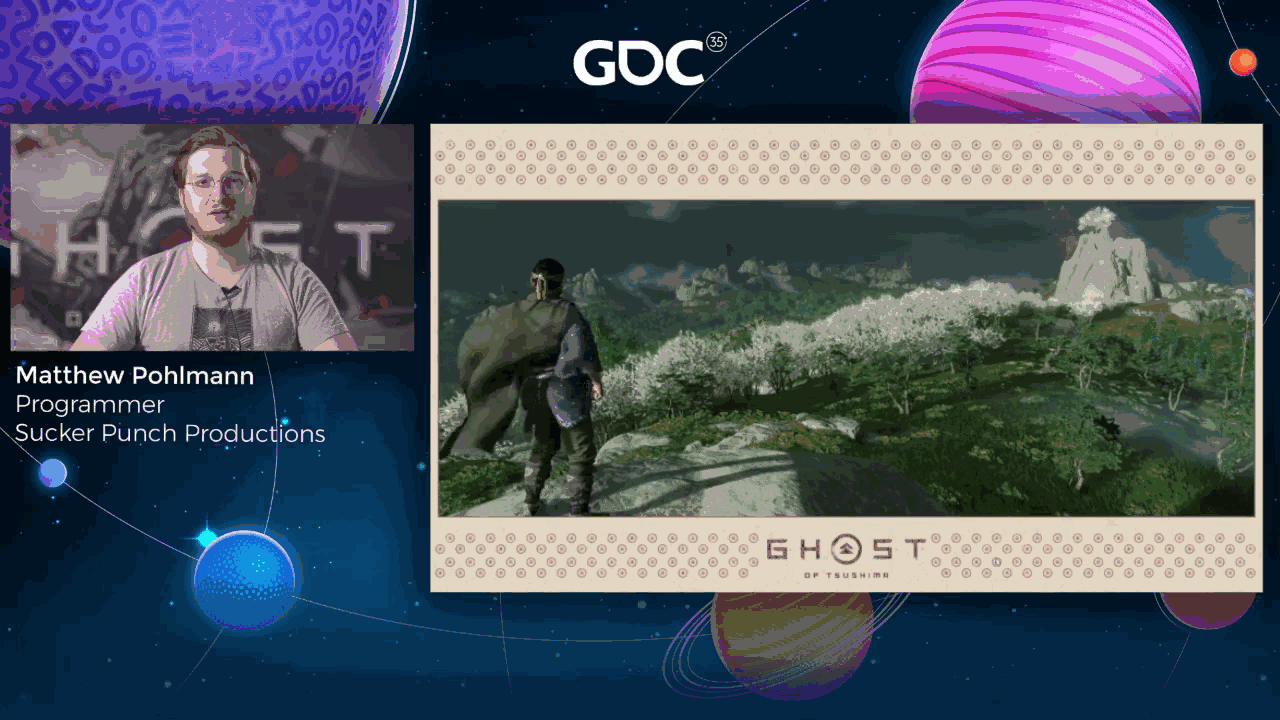
Kosushima is an open-world game that takes place in 13th-century Japan on Sushima Island. You play as the samurai Jin in your quest to take back the island from invading Mongols. The island of Sushima is much larger than Sucker Punch’s previous games. The playable area is roughly 30 km², more than 11 times the playable area of Seattle in Infamous Second Son. It’s also much more organic compared to the concrete cityscape of Infamous. Sushima is full of dense vegetation and long sightlines. We needed a toolset and runtime tech capable of populating this.

Populating and rendering this massive world, none of which existed prior to Ghost. Beyond the problems of scale, we had two other issues. Our studio is relatively small. Our programming team is less than 25 coders, and our engine only runs on PlayStation dev kits. If we wanted to author content in the context of the actual game world, we need all the tools we produce to run on PS4 Pro development hardware, and we need to invest heavily in tools that could edit at large scales and take advantage of procedural generation.

At launch, Ghost shipped with over 2.8 million procedurally placed assets and three gigabytes of texture data.

Slide 4 — 00:01:25

📌 要点汇总

（过渡内容，无关键要点）

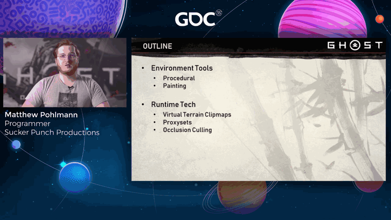
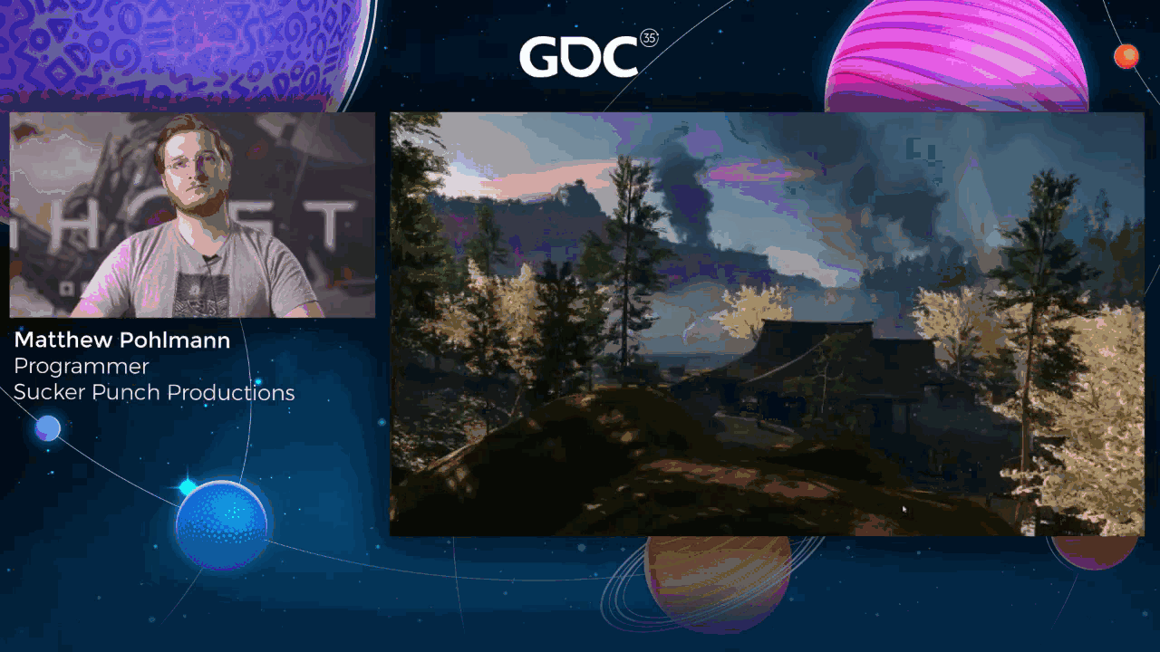
Today, I’m going to talk about two main things: the tools we developed to build Ghost’s environment, and a collection of runtime systems we built to meet our artistic and performance goals for the game. Before I begin, I’d like to start off with some screenshots I took flying.

Slide 5 — 00:01:39

📌 要点汇总

（过渡内容，无关键要点）

Around Sushma Island to demonstrate the variety of results that we achieved.

Slide 6 — 00:01:50

📌 要点汇总

开发了四款用于构建Sushima Island环境的工具，分为程序化工具和绘画工具两类
工具主要用于Ghost项目的环境创作流程
强调了工具在环境设计中的核心作用

First, let’s talk about the tools we built for authoring Sushima Island’s environment. We developed four main tools for Ghost that fall into two categories: procedural tools and painting tools.

Slide 7 — 00:01:59

📌 要点汇总

提供表达式编辑器，支持创建与地形相关的材质表达式
增长工具可将资产放置在地形上，增强环境表现力

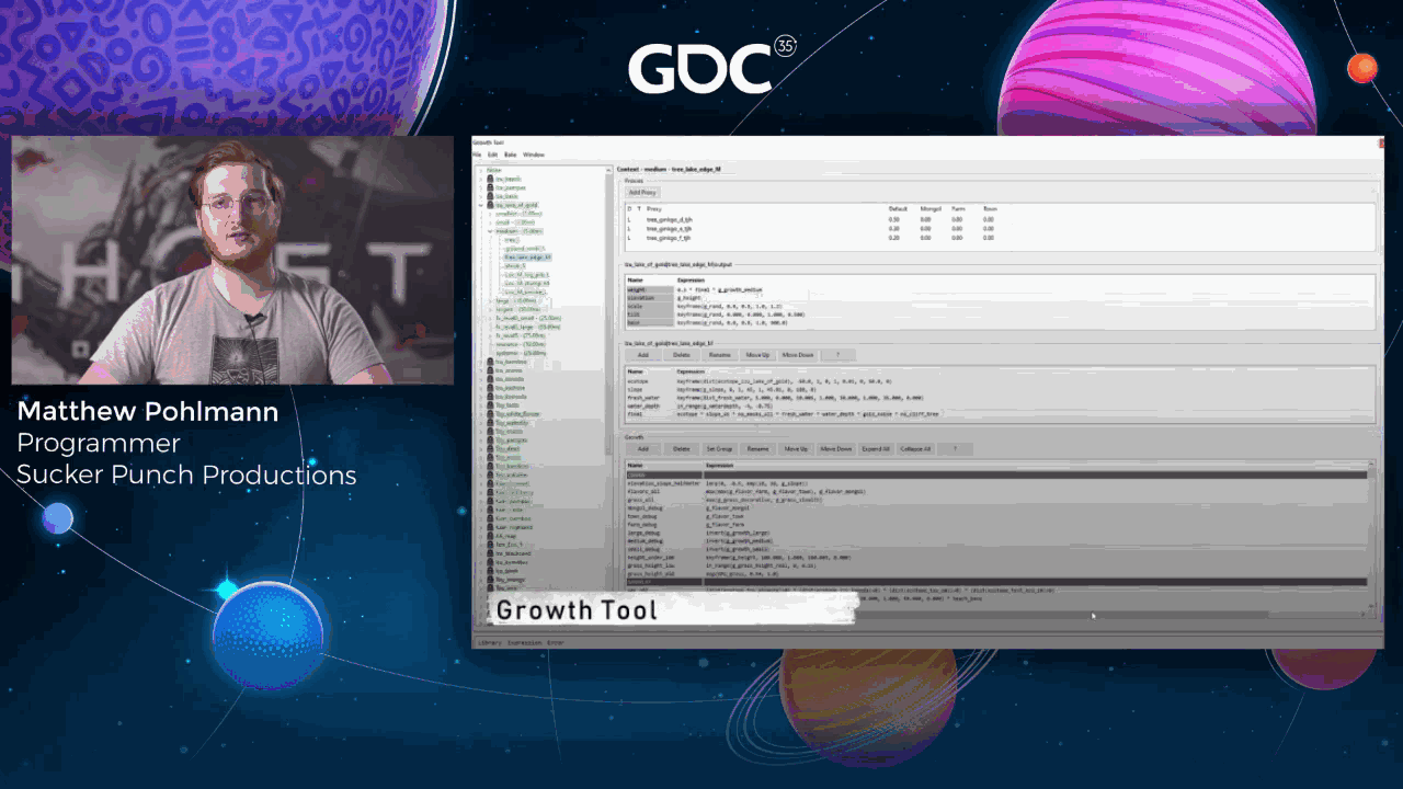
First is the expression editor, which allows users to author terrain-relative environment expressions, like terrain-blended materials. Then is the growth tool, which allows expressions to place assets on the terrain.

Slide 8 — 00:02:11

📌 要点汇总

地形雕刻工具用于编辑高度图
油漆应用用于编辑或覆盖地形图层，如混合材质和 ectope

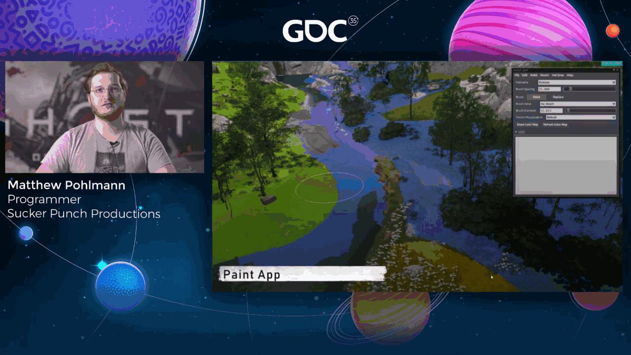
The terrain sculptor is used for editing the height map, and lastly, the paint app is used for editing or overriding terrain layers, such as blend materials and ectope.

Slide 9 — 00:02:18

📌 要点汇总

四个工具由1.5名程序员耗时两年开发，感谢同事Apura的帮助
工具运行在PS4 Pro开发套件上，用于制作大部分自然环境
地形由200米网格组成，分辨率为512 texel，对应约40厘米游戏分辨率
工具开发初期面临迭代时间长、功能限制等问题，需保持灵活性和速度
团队规模小，工具需高杠杆化，80%地形环境需程序生成，20%为手动制作
工具输出需在烘焙后保持稳定，避免输入不变时环境变化
使用10台PS4 Pro组成的烘焙农场，每晚从零开始烘焙环境数据，耗时约1小时

These four tools took one and a half coders roughly two years to develop. I’d like to thank my colleague Apura for being the extra programming help I needed to get everything done. All are in-engine tools that run on PS4 Pro dev kits and are how the majority of the natural environment is authored. We initially tried supporting the tools on base PS4 dev kits, but they just didn’t have enough extra memory.

Everything starts with the terrain. The world is a grid of 200-meter tiles at 512 texel resolution. This equates to about 40 centimeters of in-game resolution. Most terrain data is authored at this resolution, though some is lower to save on memory. My colleague Adrian’s talk goes a bit more in depth about our terrain data streaming.

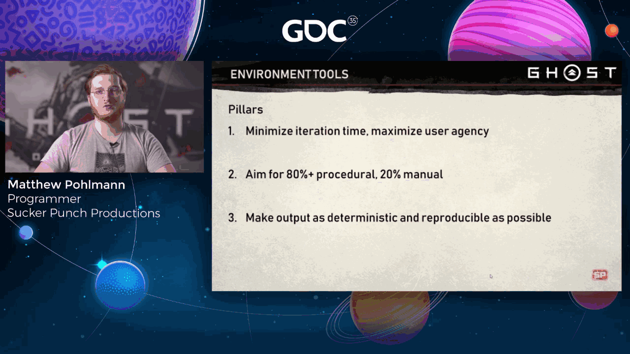
We had three main goals when building these tools. The first was minimal iteration time. Users needed to have real or near real time feedback when making changes, and we shouldn’t limit what users could express. We set out on this project. We couldn’t predict all the different types of things that we’d end up authoring using the tools, so it was important that they be flexible and fast. The first couple months of using the tools involved a huge world. As we learned what did and did not work, and what new features we’d have to add.

Second, we have a small team. The tools we built had to be high leverage across the studio. We didn’t have time to manually author everything, so we planned for at least 80% of the terrain environment to be generated procedurally, with the remaining 20% a combination of manual asset placement and terrain sculpting and painting. This excludes custom locations like towns and farms, where things were mostly authored manually and the quality bar was higher.

The output of the tools needed to be stable between bakes. Users need to be sure that nothing would change in the environment if none of the inputs change. This became extra important towards the end of the project when we started locking down the environment to prevent content breakages. We have a bake farm that uses 10 PS4 Pros to bake all of our environment data from scratch every night, which ran mostly without issues all the way until we shipped the game. A full environment bake on this farm takes about an hour on 10 dev kits, most of which is actually just waiting on streaming while moving around the world.

Slide 10 — 00:04:10

📌 要点汇总

将介绍用于程序生成的架构设计
架构是使用工具前的关键基础
涉及生成流程和系统结构的说明

Before we go into the tools, though, I need to explain our procedural generation architecture.

Slide 11 — 00:04:15

📌 要点汇总

表达式工具基于简单的函数表达式构建
表达式字节码评估器尽可能简单，因为运行在GPU上
不支持栈帧的动态分配，所有线程必须执行相同指令
操作码通常简单，如 add 或 min，但包含一些高级采样指令
表达式可访问基本数学运算等资源
后续幻灯片将讨论参考掩码和生态位概念

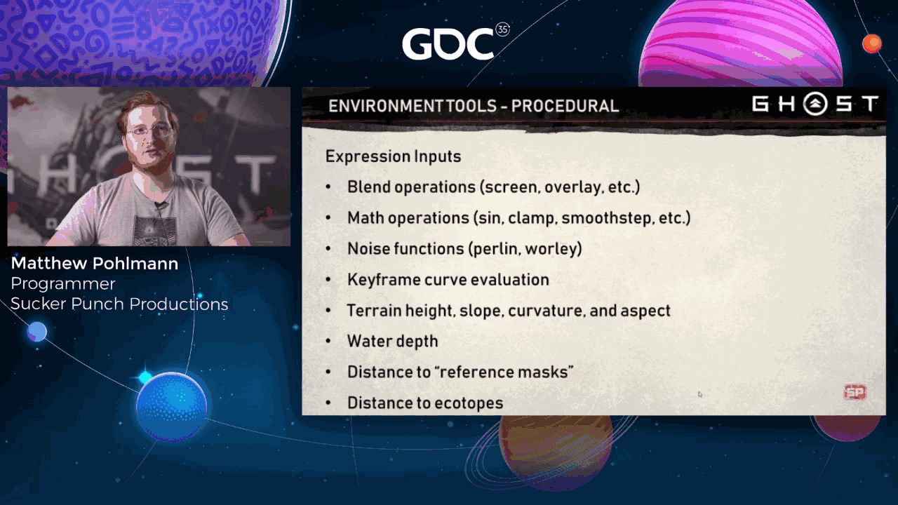
Procedural tools are built on a simple functional expression. The expression bytecode evaluator was kept as simple as possible, since it runs on the GPU. There’s no dynamic allocation for stack frames, and all threads in a wavefront must be executing the same instruction, so no dynamic branching either. Opcodes are generally simple, like add or min, but there are a few more advanced sampling instructions that simplify how artists get at important data or generate noise patterns.

Here’s a non-exhaustive list of some of the things that expressions have access to, like basic math. I’ll discuss the concept of reference masks and ecotopes in upcoming slides, as they’re extremely important.

Slide 12 — 00:05:21

📌 要点汇总

字节码评估函数接收操作数组、操作范围、关键帧数组和评估上下文，返回一个浮点数
字节码操作通过栈进行值的压入和弹出，并能从字节码中获取字面量
字节码机结构简单，便于添加新操作码
部分操作引用“hot zone”，即允许评估表达式的区域，将在后续幻灯片中详细说明

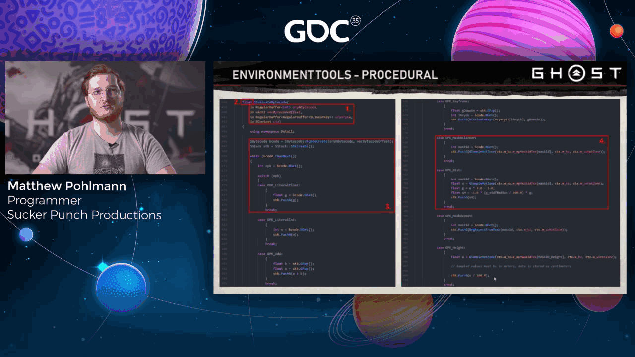
Here are some of the code snippets of actual bytecode evaluation functions. We take an array of ops, a range describing which ops to evaluate, an array of keyframes, and an evaluation context. The result is a single float. The code is pretty straightforward. We execute bytecode ops until we run out. Then the return value is at the top of the stack. Ops push and pop values from the stack and can retrieve literals from the bytecode itself as well. Because the bytecode machine is so simple, it’s straightforward to add new opcodes as necessary.

Some ops reference the hot zone, which is the area of the world where we’re able to evaluate expressions. I’ll go into more detail about the hot zone in upcoming slides.

Slide 13 — 00:05:57

📌 要点汇总

该着色器用于预览表达式输出并存储到纹理中，常用于调试
可将结果纹理绘制到屏幕或叠加到地形上
评估表达式前必须在评估上下文中设置位置
所有表达式评估默认基于地形上的点
exprSet 对象包含所有编译后的字节码和相关数据

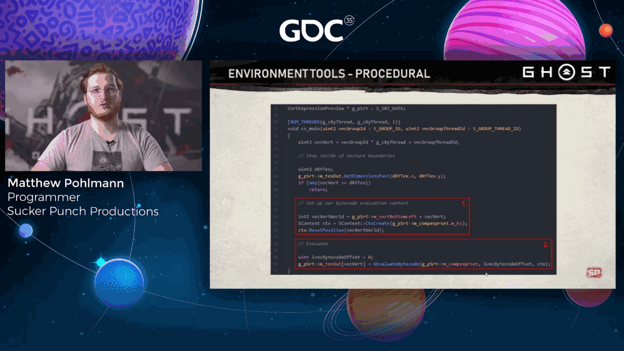
This is a simple shader that previews the output of an expression and stores the result into a texture. We generally use this to debug the output of individual expressions and either draw the resulting texture to the screen or overlay it on the terrain. You’ll note that we must set the position in our evaluation context before actually evaluating the expression.

As I mentioned before, all expression evaluation is assumed to be relative to points on the terrain, so we can do things like sample a height map. The exprSet object is the structure containing all the compiled bytecode and associated data. Data required for expression evaluation.

Slide 14 — 00:06:28

📌 要点汇总

热区是所有表达式评估的基础，覆盖3x3地形瓦片区域
热区内生成高分辨率纹理堆栈以加速表达式评估
热区随视角移动或源数据修改（如高度图）而更新

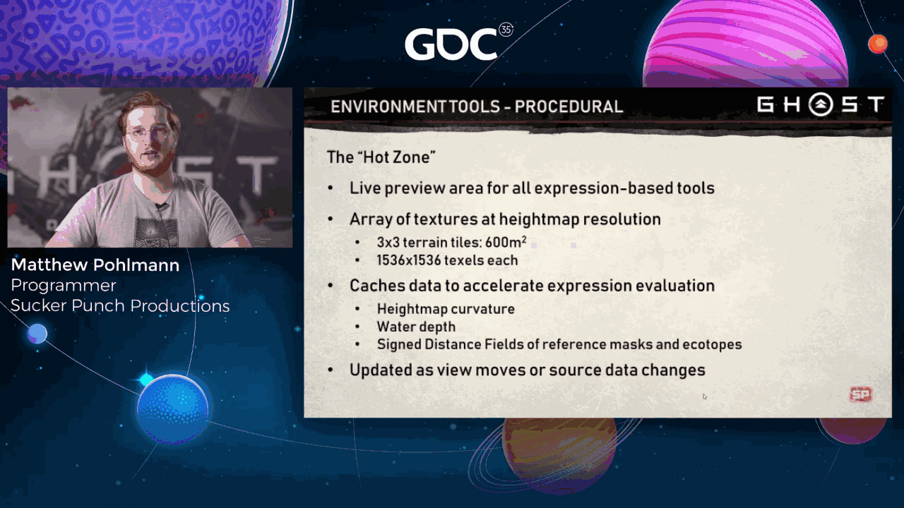
The hot zone is the basis for all expression evaluation. It’s a 3x3 terrain tile area in the world in which we generate a stack of textures at high map resolution that are used to accelerate expression evaluation. The hot zone is updated as the view moves to cover new 3x3 tile regions, or when the tools modify source data like the height map.

Slide 15 — 00:06:48

📌 要点汇总

使用青色方框标记热区表达式所在区域
第一个表达式过滤距离海洋至少40米的区域
第二个表达式过滤距离河流25米的区域

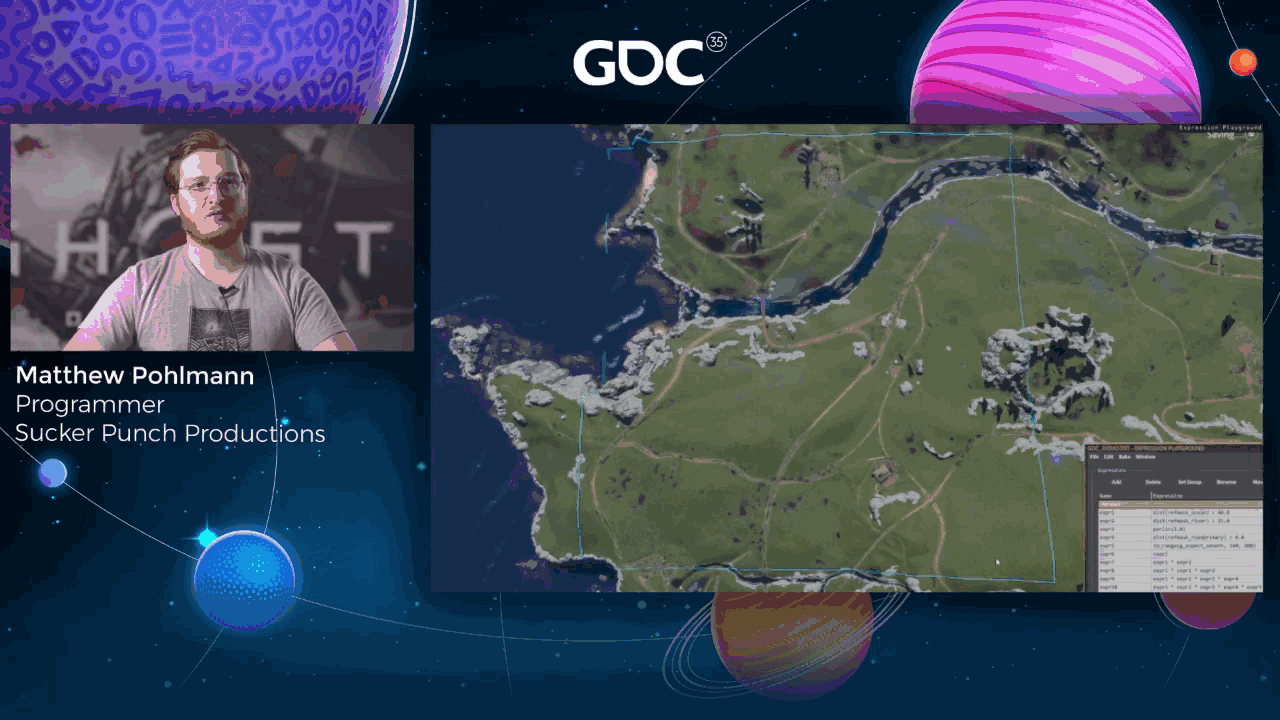
In this image, the region marked by the teal square is where the hot zone expression is in this view. Here, I’ve set up some basic expressions to demonstrate how things work. The first expression masks out areas that are at least 40 meters away from the ocean. The second masks areas 25 meters away from rivers.

Slide 16 — 00:07:10

📌 要点汇总

使用扩展的 Perlin 噪声技术来遮蔽道路区域
该方法有助于提升图像细节和真实感

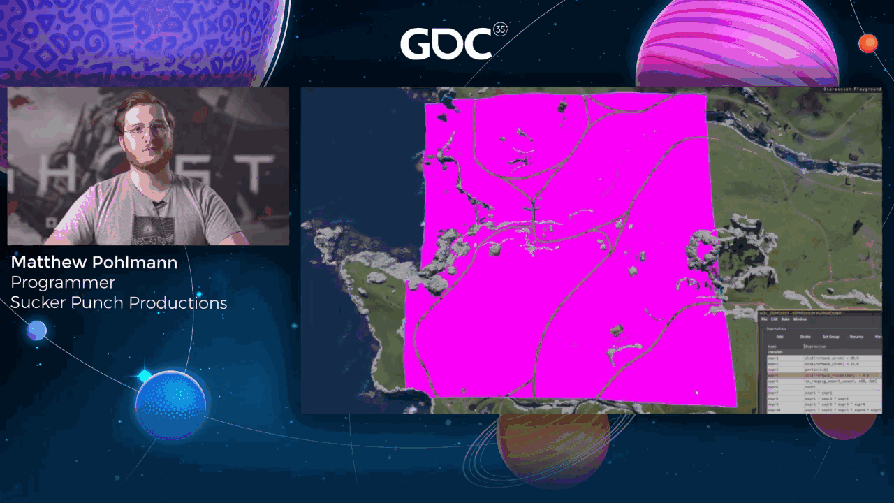
The third is some scaled Perlin noise, something that masks out roads.

Slide 17 — 00:07:16

📌 要点汇总

识别朝南的坡地，并将它们合并显示。

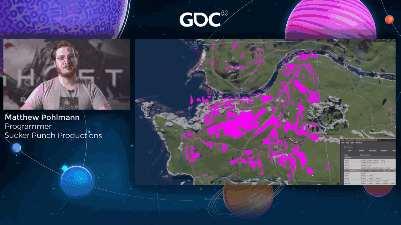
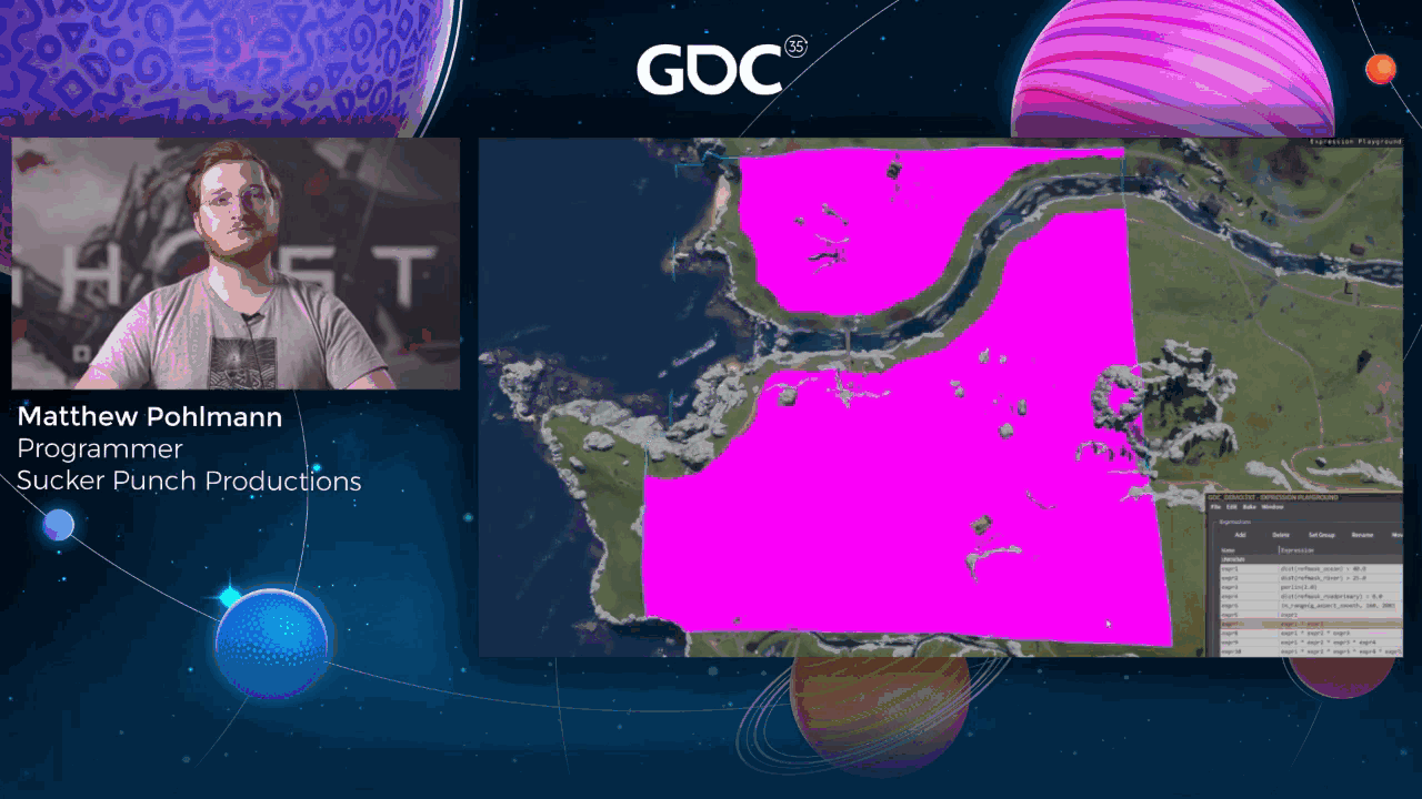
Identifying slopes that face south, and here’s what it looks like as I combine them all together.

Slide 18 — 00:07:22

📌 要点汇总

(Content too short, no key points)

。

Slide 19 — 00:07:27

📌 要点汇总

热区会随着角色在场景中的移动自动更新位置
视频展示了相同表情在不同视角下的表现
实时定位技术确保热区与角色位置同步

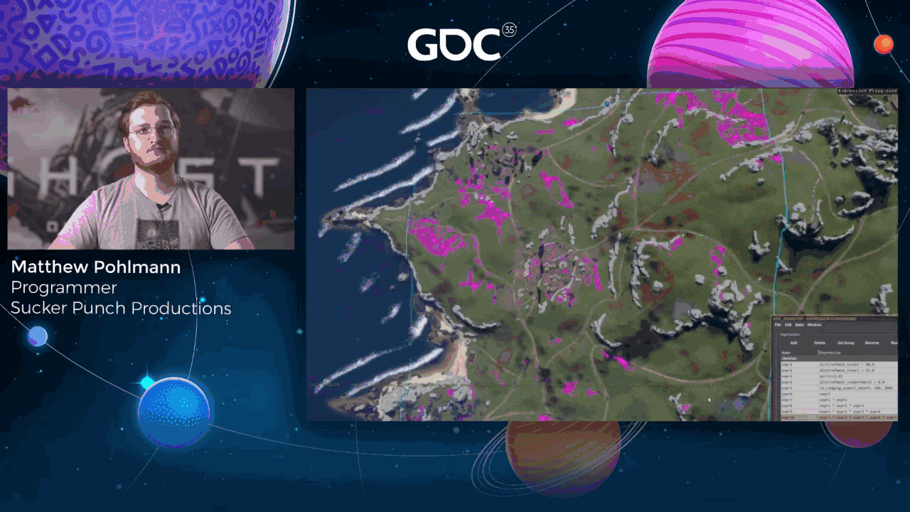
And here’s another video showcasing the same expression, but as I move around in the world, you’ll note that the hot zone updates automatically as the location moves.

Slide 20 — 00:07:44

📌 要点汇总

Reference masks 是热区更新时生成的二进制掩码，用于生成 signed distance fields (SDF)
SDF 的最大半径限制为 50 米，因内存和精度限制，使用 8 位纹理，宽 1,536 texels
部分区域需处理超过 50 米的 SDF 距离，需采用创意方法解决
“implicit” 掩码根据海洋或道路脊线自动生成，用于调试和渲染文明参考掩码
文明掩码以透明红色几何体形式存在，用于热区激活时生成 SDF

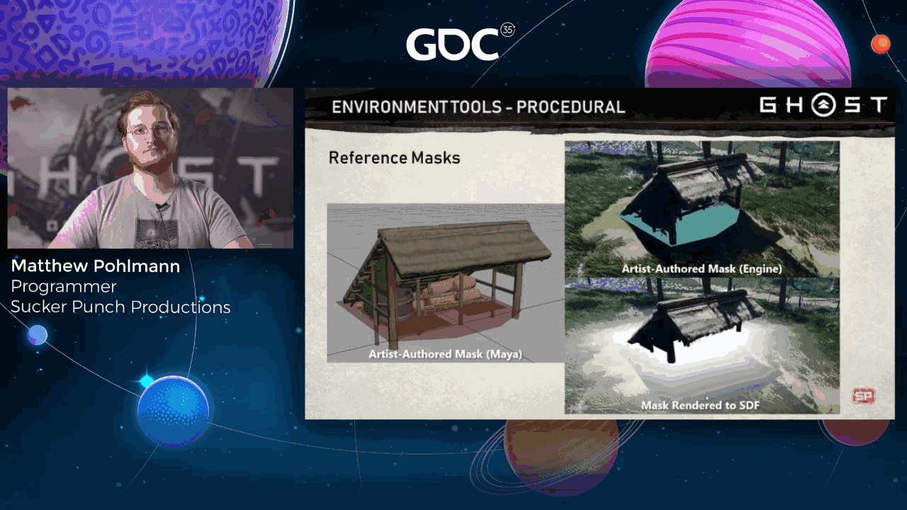
Reference masks are the second major part of the hot zone after heightmap data. They are generated when the hot zone is updated by gathering up simple geometry authored on assets or in the world and splatting it into large binary masks, which are then processed into signed distance fields to be read by expressions. We choose a max of 50 meter radius for SDFs due to memory and precision constraints. Each SDF is 1,536 texels wide and is an 8 bit texture, and we just couldn’t afford to make them 16 bit or any larger. This turned out mostly fine, except for a few places where we had to get creative with distances greater than 50 meters away from the ocean.

The masks marked implicit are generated automatically based on either where the ocean is or road spines. The source asset here has a mask marked as civilization, seen as the transparent red geometry. This mask is made available as debug data to the engine tools, which is then rendered into the civilization ref mask when the hot zone is active. Here it is in the engine. And then rendered to the SDF.

Slide 21 — 00:08:46

📌 要点汇总

使用 GPU 上的 jump flooding 算法生成 SDF，支持同时计算内外距离
SDF 距离范围从 -50 米到 +50 米映射为 0 到 1 的纹理值
热区边缘 50 米范围数据无效，避免跨瓦片地图缺失问题
游戏烘焙数据时只使用热区中心瓦片结果，避免边缘数据问题
Ecotopes 是用于定义世界区域的模块，支持如海滩、森林等分类
最终发布包含 42 个 ecotopes，远超最初预估的 20 个
Ecotopes 地图是手工绘制的，但最初每个 ecotope 都有独立地图
由于 PS4 内存限制，最终只保留一个全局 ecotope 地图用于特殊资产
每个热区只生成实际存在的 ecotype SDF，其余用黑色纹理替代
热区各图层分辨率一致，总数据量约 70MB，不包含原始源数据
高度图复制并 d-tiled 成热区大小纹理，消除地形瓦片边缘伪影

We generate our SDFs on the GPU via a variant of the jump flooding algorithm, which you can read more about in the jump flooding paper. We use a modified version that only cares about a single feature or classification, since our masks are binary, and we calculate both inner and outer distances simultaneously. Those are the distances from outside texels to the edge, and then inside texels to the edge. The distances are mapped from negative 50 meters to positive 50 meters to a zero to one range in the texture, and then remapped when sampled by expressions. Our SDFs have a radius of 50 meters. There’s also a 50-meter band around the edge of the hot zone with technically invalid data. This is because it could be missing potential maps from the next tiles over that aren’t part of the hot zone. For preview, this is mostly fine, but when we bake out actual data for the game, we avoid this by calculating everything in the hot zone and then only taking the results from the center tile.

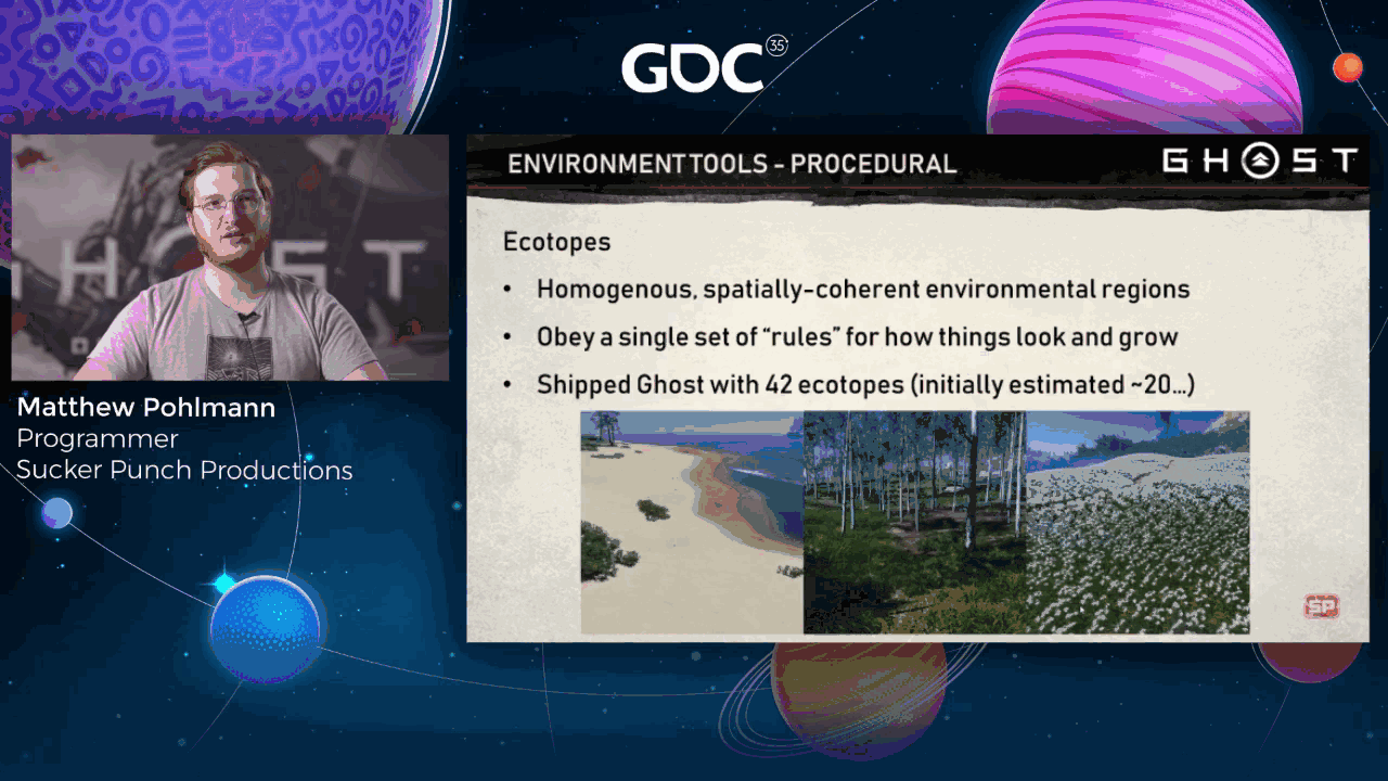
Ecotopes are the building blocks for how we designate regions of the world that have common expressions. They’re really just a way to group concepts like beach or forest so that the expressions can react appropriately. Here’s some examples. There’s a beach, a birch forest, and pampas fields. You’ll notice that we shipped with 42 ecotopes, much more than the initial 20 that we estimated. The ecotope map describes where all of our ecotopes are in the world. It was entirely hand painted over the entire island, though I’ll go into a bit more detail when we talk about our painting tools. We originally started with one ecotope map per ecotope. Ecotopes could freely overlap and be placed anywhere, but we soon ran into issues. Overlapping ecotopes were hard to write consistent rules for, and having to load one map per ecotope just wasn’t an option due to memory constraints on the PS4. The one exception is the special implicit all-map ecotope that encompasses all landmass of the island. We use this for exceptional assets that aren’t necessarily tied to any environment rule set.

We still want our users to be able to make distance queries against ecotopes, though, so we still need to generate one SDF per ecotope. But if we couldn’t load one texture per ecotype, how could we generate one asset per ecotype? And the answer is we don’t. We rely on the fact that usually a hot zone-sized region will contain a small subset of all ecotypes. When updating the hot zone, we pre-process the ecotype map to determine which ecotypes are actually present, and then only generate ecotype SDFs for those. The remaining ecotypes get replaced with pointers to a one-by-one black texture, so that expression queries still work.

Here’s the final breakdown of all the layers in the hot zone. Each layer has the same resolution, so altogether we’re allocating about seventy megabytes of data. This is just for the hot zone, though, and doesn’t include all the original source data, like per-tile height maps, ecotope maps, etc., that get loaded in cache to generate the hot zone. Note that we make a copy of the height map, but d-tiled into a single hot zone-sized texture. This removes artifacts at the edges of terrain tiles where we’d get bad normals and simplifies expression lookup.

Slide 22 — 00:11:31

📌 要点汇总

Expression Editor 是用于程序生成地形纹理的工具
最初用于创建地形混合材质，后续逐步增加功能层
新功能层添加相对容易，例如将环境音频地图输出集成到 Expression Editor 和 Paint App 仅耗时一天
几乎所有输出都可以通过绘画工具手动调整
输出分辨率根据需求和内存限制，可为高度图分辨率或更低

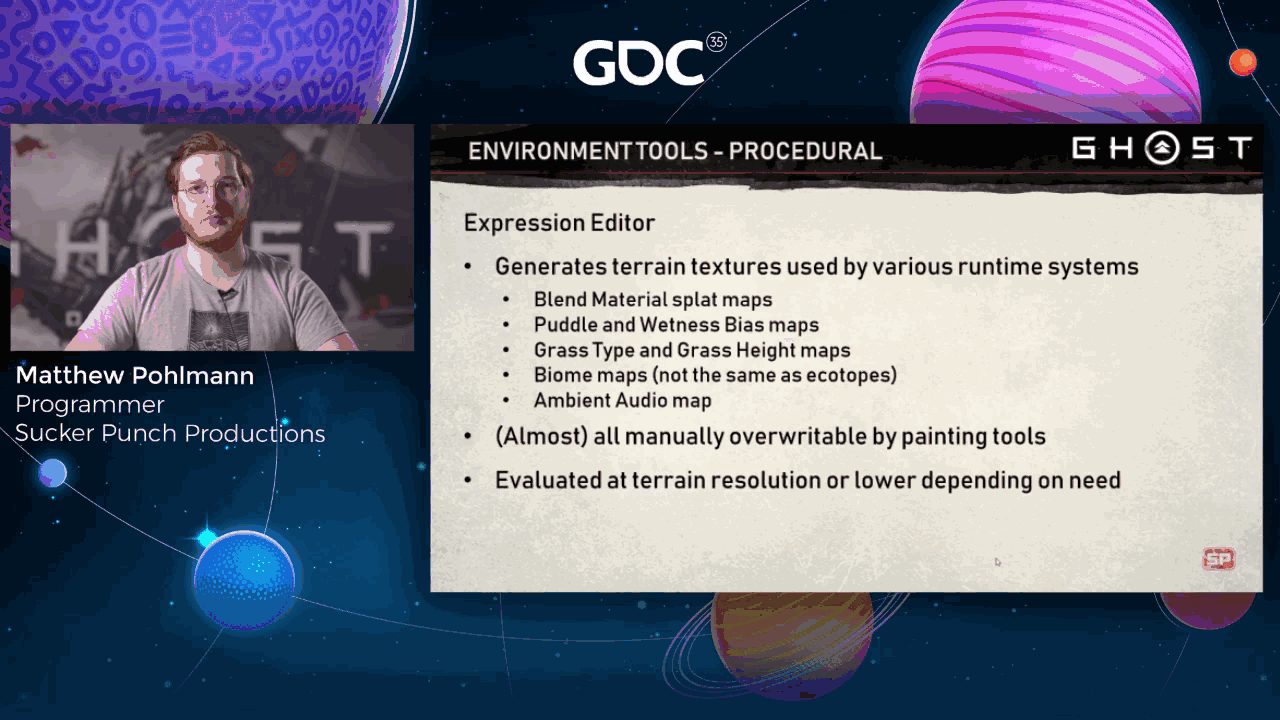
Now that we’ve talked about the basis for our procedural tools, let’s talk about the tools themselves. The first is the Expression Editor. The Expression Editor is an interface for procedurally generating terrain textures. It started as a way to author just our terrain blend materials, which I’ll talk about later, but we added additional layers over time. In the end, it was relatively easy to add new layers. For example, adding the ambient audio map output to both the Expression Editor and Paint App took me about a day’s worth of work. Almost all of the outputs are manually tweakable by the painting tools. So that artists have control when they need it, and output resolution is either heightmap resolution or lower, depending upon need and memory constraints.

Slide 23 — 00:12:07

📌 要点汇总

左侧面板显示每层的最终输出表达式，右侧是可被引用的共享表达式工具箱
混合材质溅射图通过多个材质的 alpha 混合生成最终效果，支持最多三个材质在同一 texel 混合
湿度输出包含两个纹理，分别用于静态水洼和全局湿度偏移
草地类型输出控制运行时生成的草地类型，根据 alpha 混合结果选择贡献最大的类型
草地高度输出控制运行时草地基础高度，但因假设错误导致实现复杂且问题频发
生态带地图输出是生态图的低分辨率近似，用于影响运行时系统行为
环境音频地图用于生成环境音效，如鸟鸣、水流等，音频总监 Brad Meyer 有相关博客和演讲
部分输出为零，表示某些小生态带手动绘制在少数需要的位置
草地高度输出应按草地类型拆分，以减少复杂度和问题

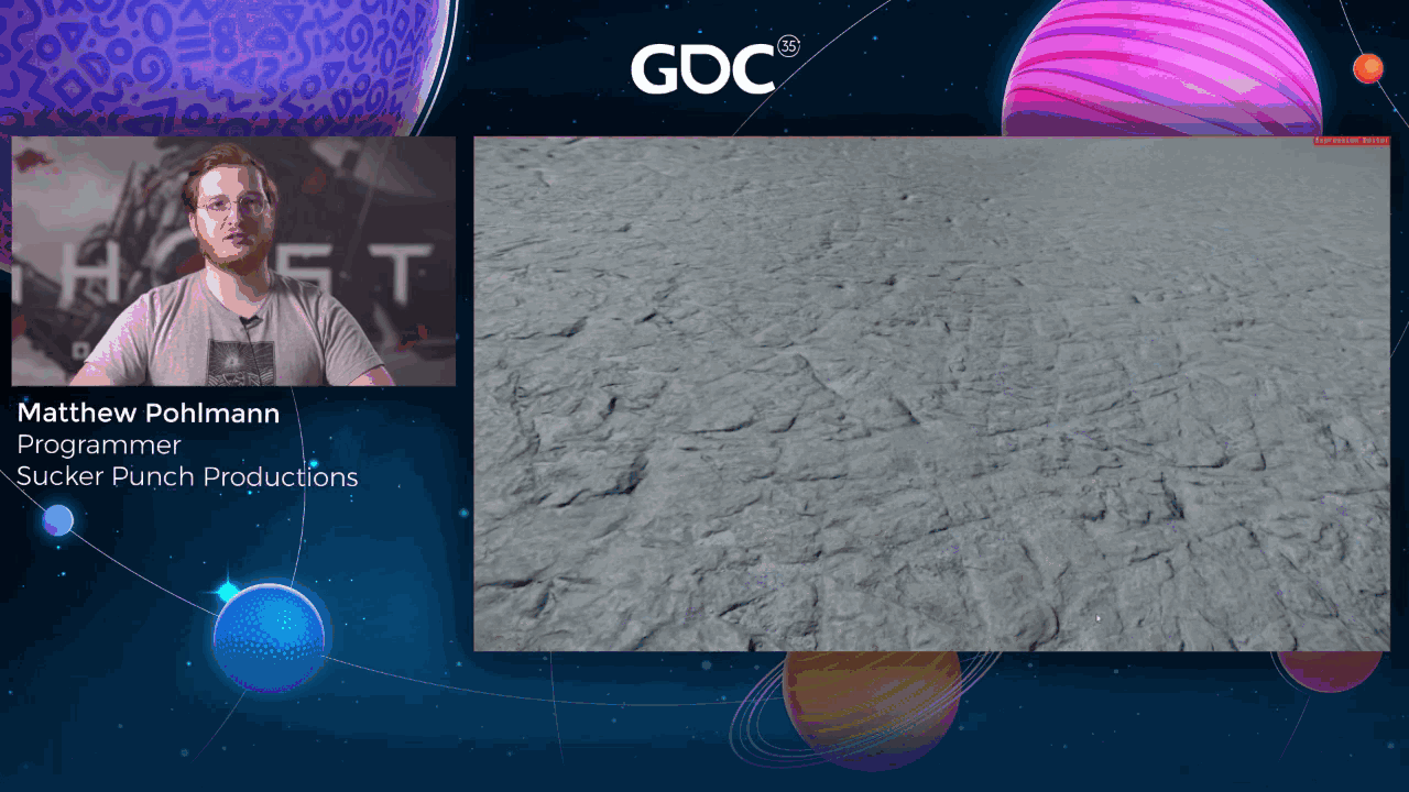
Here’s the tool itself. On the left pane, we have all the final output expressions for each layer, and the right pane has a toolbox of shared expressions that can be referenced by the left pane. The first output are our blend material splat maps. We have a stack of train materials that get alpha-blended together to form the train’s final look at runtime. We support three materials blending in the same texel, so we evaluate expressions down the stack until their final alpha contribution sums to one. At which point, we early exit the evaluation loop, changing the order of materials here changes the output.

The wetness outputs are two separate textures. The first adds static puddles to the world, while the wetness bias output is a static bias to the global dynamic wetness level. The grass type output controls the type of runtime-generated grass that gets placed per heightmap texel. These are evaluated similarly to the blend expressions, but there’s only a single output per texel, so we take the type with largest contribution after the alpha blend reaches 100% contribution. For more details about procedural grass, see my colleague Eric.

Grass height output is a single 0 to 1 output controlling the base height of procedural runtime grass. We did this thinking that the base pattern of grass would be relatively similar between all grass types, but this turned out to be a bad assumption. This expression has to modify grass height for all types of grass, so it’s incredibly complex and was a constant source of problems. In retrospect, we should have split it up per grass type.

The biome map output is a rough lower res approximation of our ecotope map. It’s used by a couple of runtime systems to change their look or behavior based on the player’s location in the world. For example, particles might choose to use red leaves or grass blades depending upon biome. You note that some of the outputs are just zero. These were small enough biomes that they were painted in manually in the few locations that they were needed.

The ambient audio map is sampled by our runtime ambient system to generate sounds in the environment, like birds chirping or water splashes and rivers. If you’re interested in audio stuff, our audio director Brad Meyer has written some blog posts, and we’ll be giving a talk about sound design in Ghosts of Tsushima as well. Here’s a short clip where I enable each of these expression editor outputs and turn.

Slide 24 — 00:14:09

📌 要点汇总

从空白的 splat maps 开始构建基础 bedrock 层
添加了地形材质以增强视觉效果
引入了水洼和湿度过滤效果
最后添加了草地以丰富场景细节

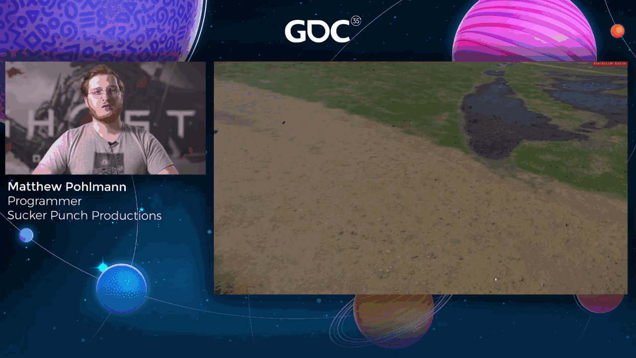
I started with a base bedrock layer with empty splat maps, but then added in terrain materials. I then added in some puddles and a wetness bias. Lastly, I added in some grass.

Slide 25 — 00:14:24

📌 要点汇总

将草的高度从默认值 1.0 修改为更有趣且合理的数值
生态系统地图用于粒子系统的输出控制
摄像机连接的粒子系统根据所处生态系统改变输出效果
竹林中显示绿色竹叶，黄金森林中显示黄色叶子

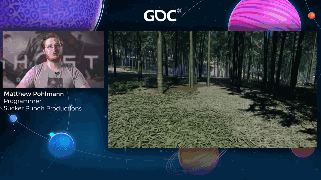
And then modify the grass height from the default 1.0 to something that’s a bit more interesting and plausible. Here are a couple of quick videos showing how the biome map is used by particle systems. We have a particle system attached to the camera that changes its output depending upon what biome you’re in. In this first video, I’m in a bamboo forest, so we get green bamboo leaves. But here in the golden forest, I get yellow leaves.

Slide 26 — 00:14:49

📌 要点汇总

GPU 上表达式编辑器对每个图层的评估时间有具体数据
通过分地形瓦片评估，九帧内完成热点区域评估以保持交互性
表达式复杂度在项目后期呈指数级增长，影响迭代效率
同时只能编辑一个表达式，但评估时间仍超出预期
低分辨率生物群落和音频地图评估速度更快
高分辨率的 alpha 混合和草类型评估耗时远超预期
正在考虑多种解决方案，但当前状态已被认为可接受

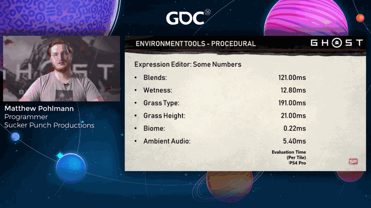
Here are some numbers representing how long it takes for the expression editor to evaluate each layer on the GPU. We break up evaluation by terrain tile and evaluate the entire hot zone over nine frames in an attempt to keep things interactive. The complexity of some of these expressions grew exponentially towards the end of the project, which made it more difficult to iterate.

Overall, it’s not too bad as you can only physically edit one expression at a time, but it is longer than we’d like. The lower resolution biome and ambient audio maps obviously evaluate much more quickly, but the complex evaluation scheme of alpha blending at full resolution for blends and grass type make them take way longer than we initially expected.

We’re considering various solutions to this problem, but the current state of things was deemed acceptable.

Slide 27 — 00:15:28

📌 要点汇总

Ghost 的 growth 工具用于在开放世界中生成大量资产
最初仅用于放置树木，后扩展至 PFX、资源和系统性地点
发布时生成了 280 万个资产
若人工放置每个资产需 15 秒，需超 5.5 年完成，且无错误和迭代

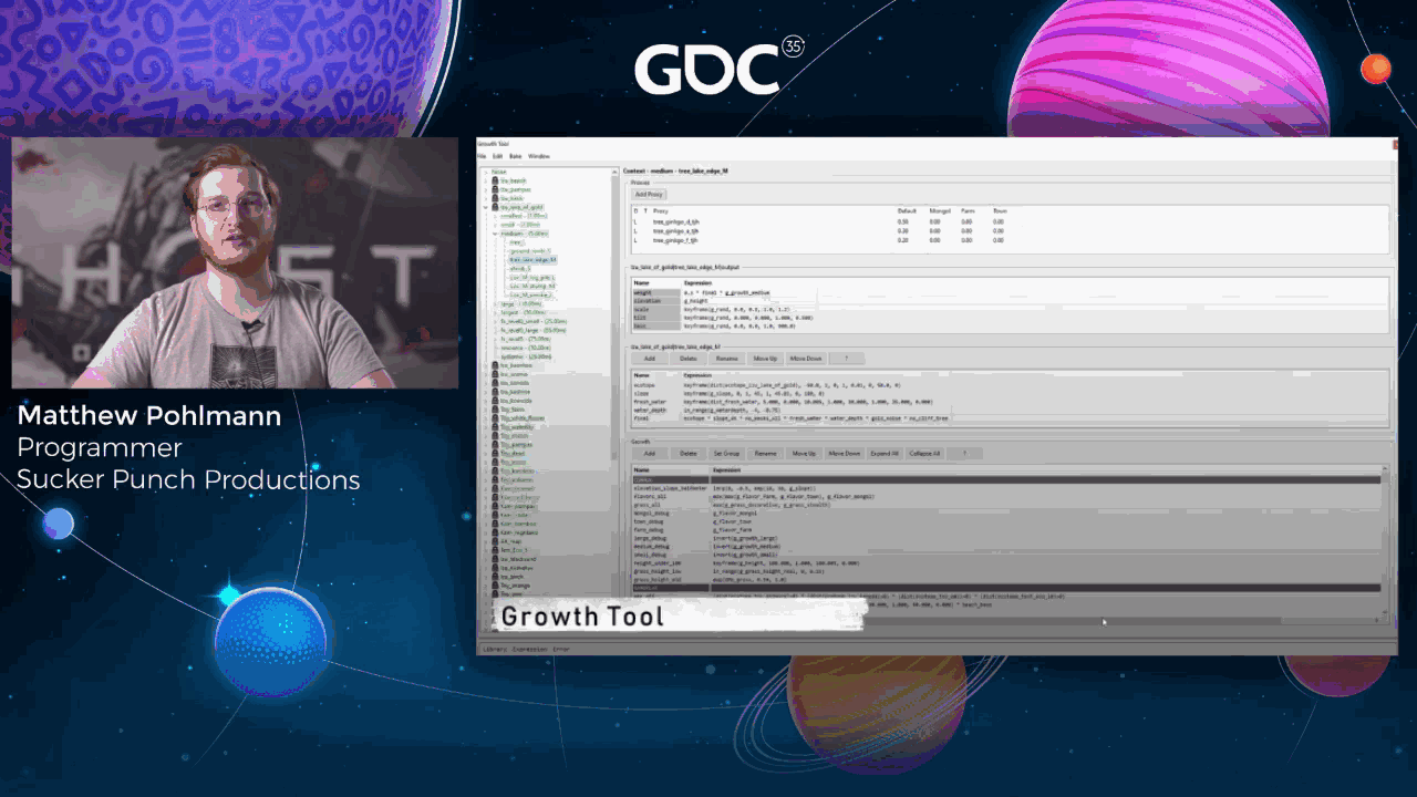
For Ghost, the second procedural tool we built is the growth tool, whose purpose is to populate the terrain with assets. The growth tool is how the vast majority of assets in the open world are authored. Originally, all it did was place standard assets like trees, but soon we realized it would be just as useful for placing other types of assets like PFX and resource and systemic sites, which are seed locations used by the runtime to dynamically spawn resources like bamboo or systemic encounters like roving Mongol warbands. At launch, the growth tool was responsible for 2.8 million grown assets. Some napkin math estimates say that if it took 15 seconds to place a single asset in the world, it would have taken over five and a half years for an environment artist working full time to populate the same world. And that’s with zero mistakes and zero iteration.

Slide 28 — 00:16:12

📌 要点汇总

资产生成工具采用分层结构，从抽象的生态位（ecotope）到具体的资产（如树A）
生长规则设定后，只需修改生态位地图即可生成新资产
资产在网格上生成，共有10种不同网格类型，包括用于特效的特殊网格
每个“生长角色”（growth role）包含特定资产类型的表达逻辑和权重计算
角色权重决定最终资产属性（如比例、旋转），权重总和不为1时可能生成空格
资产权重可通过“风味地图”（flavor map）进行调整，如蒙古地区树木数量变化
支持调整资产的四个属性：高度（elevation）、比例（scale）、倾斜（tilt）、基础旋转（base rotation）
资产放置在不同大小的紧密排列的圆形网格上，最终位置通过噪声函数进行偏移
GPU处理每个网格单元，计算角色权重、选择资产并转换为最终变换数据
若权重总和大于1则归一化，小于1则自动补充“无角色”以确保总和为1
每个线程将选择的资产ID和变换数据写入数组，供CPU读取使用

The growth tool was designed as a hierarchy, from more abstract concepts like ecotope to concrete assets like tree A. At the highest level, we have ecotopes, then the placement grid type, growth rules, and then individual assets. As mentioned earlier, ecotopes describe a particular environmental region, like birch forest. Once growth rules are set up for an ecotope, all you have to do is modify the ecotope map, and you’ll get an entirely new set of assets. Assets are grown on a grid with each ecotope, and we have a total of ten different grids to choose from. There are basic ones like small, medium, and large for standard assets like trees, but a couple special ones for other purposes I’ve already mentioned, like the effects. I’ll go into more detail about how these grids work in a little bit.

A growth role contains all expression logic for a particular archetype of asset, like large tree. Expressions are evaluated to determine this role’s weight with respect to other roles in its grid type. The chosen role then evaluates some further expressions that determine the final properties like scale and rotation. The tool allows for a set of supporting per-role expressions for organizational purposes, and also has access to a global set of common growth expressions. Finally, roles choose. Roles contain a list of actual assets that gets placed into the world. When a role is chosen, we choose a random one of these assets based on a weighted random choice. Note that the weights don’t necessarily need to sum to one. If they don’t, there’s a chance you get nothing at that grid cell, and it’ll remain empty.

Lastly, asset weights can be modified based on a painted flavor map. This allows you to expose things like the number of tree sums increases as you enter Mongol territory relative to normal trees. More on this later. We support modifying four properties of assets: elevation, scale, tilt, and base rotation. Elevation is useful for sinking assets into the terrain on steep slopes, but was also used for things like rice paddies at water level by placing rice paddies at water level rather than on the terrain. Scale is a single uniform value rather than a three-component scale for simplicity, and to ensure that assets wouldn’t look weirdly stretched. The tilt property describes whether the asset faces along the global up axis or whether it should match the terrain normal. And lastly, the base rotation property specifies the 360-degree rotation about the up axis.

These properties are combined in the growth computator after being evaluated into the asset’s final transform. Assets are placed on a grid of packed circles of different sizes that tile over the entire world. The final location of an asset and where we evaluate all the expressions is a point jittered away from the center of each of these cells. This approach produces seemingly pleasingly random results and is relatively simple, though it took some fiddling to find the right maximum jitter amounts to feel natural. We currently use between 10 and 40% of the cell’s radius, depending upon the grid size.

I’ll now describe the algorithm used to place assets and growth. For each tile, we dispatch work to the GPU that does the following: each center point of a grid cell gets jittered to its final position using a noise function taking the point’s location in world space as a seed. All role weights for this particular ecotope and grid type pair are then evaluated as expressions at each point. If the point is no longer in the ecotope, it gets discarded automatically. This is an implicit step, as points outside the ecotope will have a role weight of zero. If the point is no longer in the ecotope, it gets discarded. We then choose a random role amongst the surviving roles, weighted by their weight expression output.

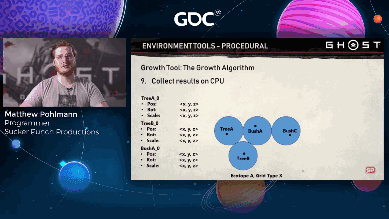
For cells where the sum is greater than one, we renormalize the weights against the actual sum. For cells where the sum is less than one, an implicit no role is added to make up the value up to one. This makes it possible for no role to be chosen at all. Now that we know our role, we choose a random asset from the list of all assets in this role. These also don’t have to sum to one. If the sum is less, then there’s a chance that no asset is chosen. We then evaluate our output property expressions for elevation, scale, tilt, and base rotation. Convert these properties to actual transform data, and then lastly, each thread writes its chosen asset ID and transform to an array that gets read back on the CPU. As an aside, we actually write a proxy set instance structure, which I’ll talk more about in detail later in the talk.

Slide 29 — 00:20:37

📌 要点汇总

展示了由不同角色和网格尺寸构建森林的过程
最后添加的草来自表达式编辑器而非生长工具

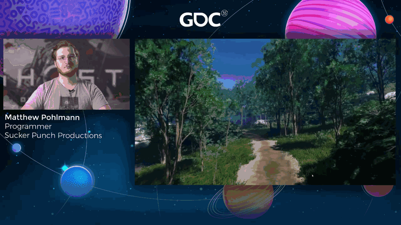
Here’s a short video made by our lead environment artist Joanna Wang that shows a forest being built up from different roles and grid sizes. Note that the grass added at the end comes from the expression editor and not the growth tool.

Slide 30 — 00:20:56

📌 要点汇总

未解决不同网格尺寸资产碰撞问题，但实际碰撞情况很少
发现碰撞问题后，手动使用绘画工具修复
环境艺术家在创作时避免了碰撞问题
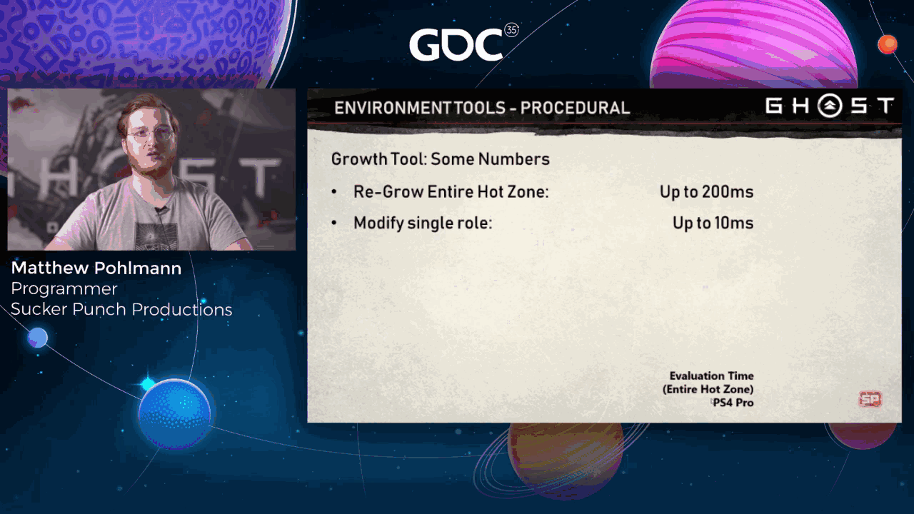
热区完全再生耗时最多达200毫秒
单个角色表达式修改仅需10毫秒
内存开销很小，热区和输出实例内存总需求约18MB

If you’ve been paying attention, you might have realized that I haven’t mentioned anything about how we avoid assets at different grid sizes colliding with each other when being placed. This was a serious concern for us at first, but we didn’t initially have time to solve the problem. It turns out we never actually solved this problem. Amazingly, we had very few assets that caused serious collision issues, and those that were noticed were fixed manually using the painting tools. Some of this might have been luck, but I believe at least part of it was due to how our environment artists authored expressions in such a way that avoided the problem in the first place.

Here are some numbers representing how long it takes for various growth operations. A full regrow of the hot zone, including all eutectoid grid sizes, can take up to 200 milliseconds. But modifying an expression for a single role can take as little as 10 milliseconds, which is the most common case. Memory overhead is also pretty minimal. We only need the hot zone, which we already talked about, and enough output instance memory for the worst-case number of generated instances, which comes out to about 18 megabytes for the entire hot zone.

Slide 31 — 00:21:52

📌 要点汇总

（过渡内容，无关键要点）

Next, let’s talk about train painting, the other half of our environment tools.

Slide 32 — 00:21:57

📌 要点汇总

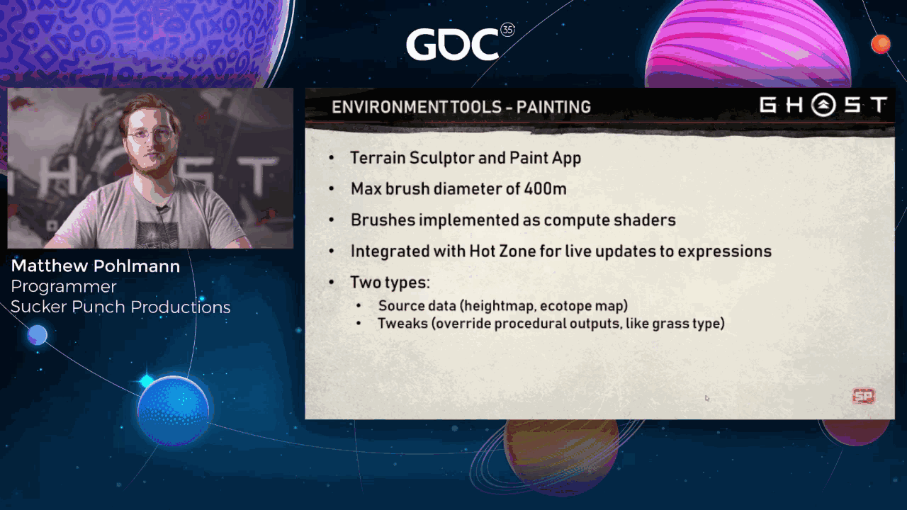
地形雕刻工具和绘画应用是两种主要的绘画工具，最大画笔直径为400米，受限于热区大小
画笔通过计算着色器实现，运行速度快，并与热区集成以实现实时预览更新
可绘制内容包括源数据本身或对程序生成数据的调整
源数据如高度图或生态图可实时更新程序表达式

We have two paint tools: the Terrain Sculptor and the Paint App. I’ll go into more detail about them in the coming slides. Both tools have a max brush diameter of 400 meters, restricted because of the size of the hot zone. Brushes are implemented as compute shaders, so they’re super fast, and are integrated with the hot zone so that changes to source data, like the height map or ecotone map, can update procedural expressions with a live preview. Some paintable things are source data themselves, whereas others are tweaks over procedurally generated data from expressions.

First, let’s talk about the Terrain Sculptor.

Slide 33 — 00:22:28

📌 要点汇总

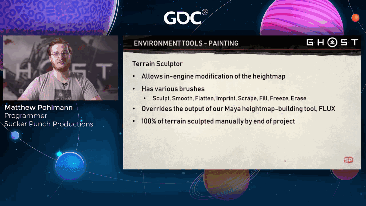
地形雕刻工具支持在引擎内直接编辑高度图
提供多种常见画笔，类似 Mudblocks 的使用体验
该工具覆盖了之前在 Maya 中使用 Flux 工具生成的岛屿地形
由于编辑反馈速度更快，几乎所有地形编辑都改用此工具完成
项目结束时，Sushima 上所有可见地形均通过此工具完成编辑

As its name implies, the terrain sculptor allows in-engine editing of the heightmap. We support a variety of common brushes that people familiar with Mudblocks will recognize. Edits using this tool override the output of our world-scale heightmap authoring tool in Maya called Flux. We built a rough version of the islands there, but once this tool was made available, almost all editing was done in the engine instead, because of the much shorter turnaround time for edits. By the end of the project, 100% of the visible terrain on Sushima was edited using this tool.

Slide 34 — 00:22:55

📌 要点汇总

PS4 上实现了基本的 USB 协议处理器，支持特定 Wacom 数位板模型
艺术家可使用带压感的数位板进行雕刻
地形编辑时，刷新发生在笔触结束，耗时较长
初始用户常保持热区激活，但表达式复杂导致性能问题
多数用户选择冻结热区，仅在满意时刷新
介绍了 Paint 工具，包含所有可绘制图层

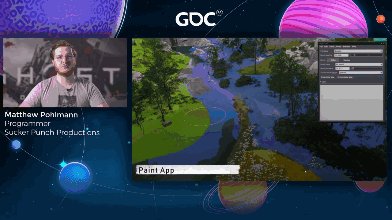
Here’s a clip of me showing off some of the different brushes, and excuse my horrible programmer art. To be fair, I am just using a mouse. As an aside, we also implemented a basic USB protocol handler on the PS4, so we could plug in a few specific Wacom tablet models for the artists. That way, they could have access to an actual tablet with pressure sensitivity when sculpting in the engine. Here’s a clip showing what happens.

If you edit the terrain while the hot zone is active, note that the refresh happens at the end of the brush stroke, and that it takes quite a long time. At first, users were able to leave this on all the time, which was awesome, but our expressions ended up being so complicated and expensive to evaluate that most people would edit with the hot zone frozen and only refresh when they were happy with their sculpting.

The last environment tool I’ll talk about today is the Paint app. This tool contains all the other paintable layers that we’ve made available to artists.

Slide 35 — 00:23:50

📌 要点汇总

Paint 应用用于编辑地形相关数据，不包括高度图
与热区集成，可实时查看绘画对表达和生长的影响
部分可绘制图层不仅用于表达，还被其他系统使用
将列出所有可编辑图层，并在后续幻灯片中逐一讲解其影响

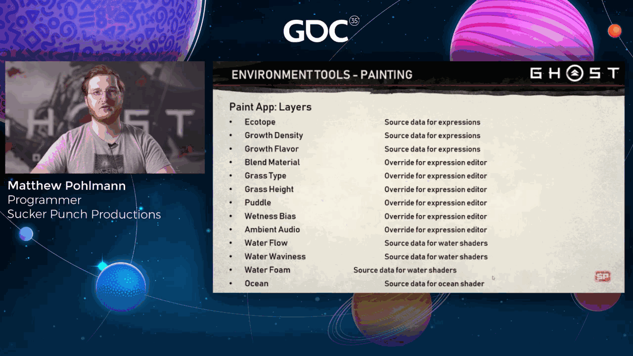
The Paint app is our solution to authoring all other terrain-relative data in the engine that isn’t the height map. Like the Terrain Sculptor, it is integrated with the hot zone, so you can see how your painting affects expressions and growth. Not all paintable layers used by expressions are source data, and some are used by systems outside the expressions as well.

Here’s a list of all of the layers that the Paint app can edit. I’ll go through each of these in the coming slides to give you a better idea of their effect on the environment.

Slide 36 — 00:24:19

📌 要点汇总

Ecotone map影响每个绘制的texel，允许用户定义生态过渡区域及其表达式。
该地图是整个岛屿由环境团队手工绘制的。
Growth density map通过大、中、小密度通道修改生长规则的最终权重。
用于调整egotopes并消除个别生成的有问题资产。
Growth flavor map影响单个资产权重，而非角色权重。
资产可配置高度，响应不同flavor，如绘制Mongol flavor时树木会偏向被砍伐状态。

The ecotone map has the biggest impact per painted texel. It allows users to define where ecotones are, and the expressions that then get evaluated at these positions. Note that this was hand-painted over the entire island as the environment team worked on new regions.

The growth density map provides an additional way to modify growth expressions. Each rule’s final weight can be modified by a specific density channel—large, medium, or small. This is used to modify egotopes along another axis, but also to paint out problematic individually grown assets.

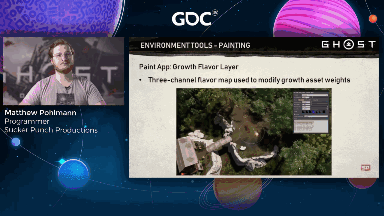
The growth flavor map is another growth modifier, but rather than affecting role weights, it affects individual asset weights. Assets can be configured with heights that respond to different flavors in the world. For example, in this video, these assets are configured to skew towards chopped down trees when I paint the Mongol flavor.

Slide 37 — 00:25:16

📌 要点汇总

混合材质可通过绘制覆盖，但Paint应用仅支持两个材质，因需存储材质ID和alpha值
四通道纹理可存储两个材质信息，支持三个材质可能增加复杂度和内存开销
手动绘制可覆盖程序化草类型和高度，也可添加静态水洼并覆盖程序化输出
水流方向和速度由水流贴图控制，该贴图在Tsushima全岛手工绘制
水波纹贴图控制非海洋水的波浪效果，最终效果在运行时根据风力调整
水泡沫层控制非海洋水的泡沫强度，海洋贴图控制海洋渲染区域
这些工具对构建Tsushima岛自然环境至关重要，大幅提升了开发效率
表达式编辑器后期变得非常复杂，编译时间接近20秒，缺乏函数和宏支持
程序化工作占比20%，但雕刻工作几乎全为手动，Ceceo岛完全手工雕刻
工具开发受限于编程资源，通常只能做到可用状态后继续推进其他任务

Procedural blend materials can be overwritten by painting to the blend material layer. I’ll note that even though our terrain supports up to three blended materials, the Paint app only allows painting two. This is because we need to store both material ID and alpha per material, so two materials can be stored in a four-channel texture. In retrospect, we probably could have supported three materials, but that would have added extra complexity and memory overhead. Procedural grass type can also be overwritten with manual painting. And so can procedural grass height. You can add static puddles to the world and override the expression editor’s procedural output. And similarly, you can modify the global wetness bias channel as well. Ambient audio can also be painted, but you can’t really see the effects of this. My colleague Brad Meyer has a wealth of additional details about audio in Ghost of Tsushima.

The water flow map is not used by expressions, but can be painted by the Paint app. This map controls both the direction and speed of non-ocean water in the game. This map was also entirely hand-painted over the entire island of Tsushima. The water waviness map controls how wavy non-ocean water looks, from a mirror finish to very wavy. The final in-game waviness is also modified at runtime, depending on how windy it is. The water foam layer controls the strength of procedural foam on non-ocean water throughout the island. And lastly, the ocean map controls where our ocean renders. Painting zero removes ocean tiles entirely, but anything larger controls the strength of ocean waves.

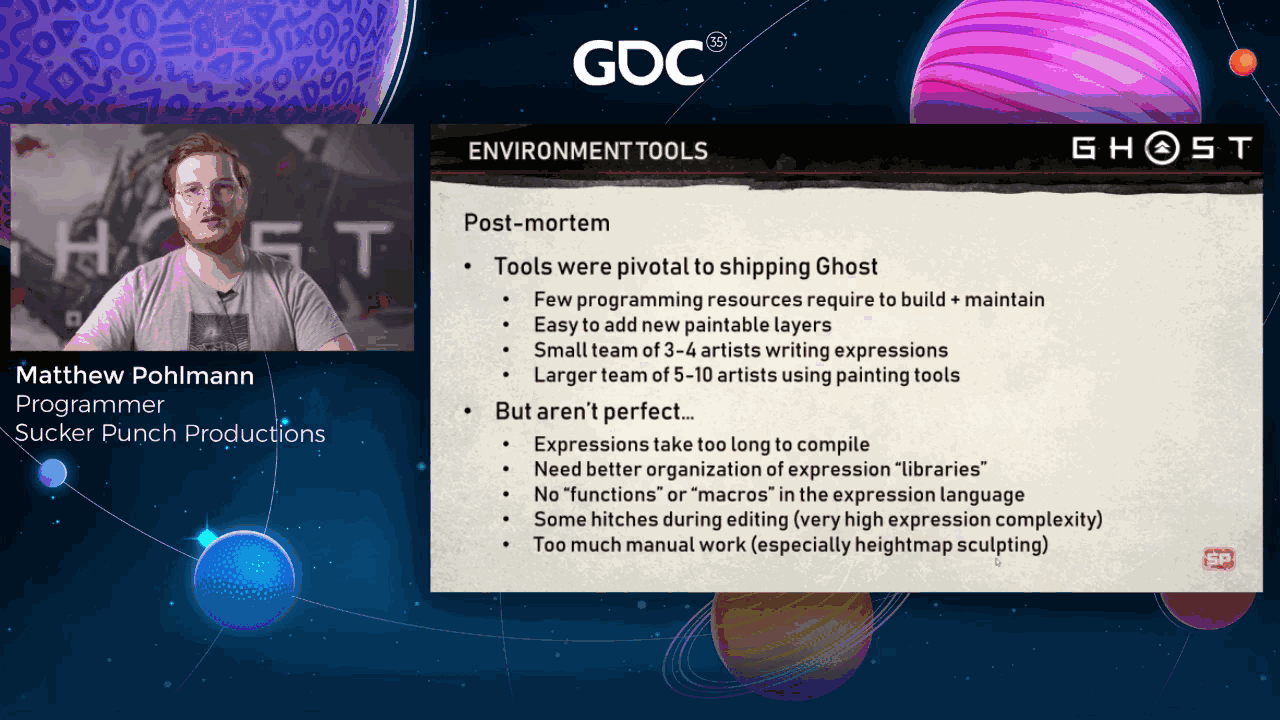
To wrap things up, these tools were incredibly important for building the natural environment of Tsushima Island, and there’s no way we would have shipped the game on time had we had to use manual placement or painting for the entire world. A very small team was able to author a huge amount of content in ways that our previous toolset just couldn’t support, and did so using tools that were also built by a very small team. Of course, not everything was perfect. Towards the end of the project, our environment expressions had grown to be massively complex. And took nearly 20 seconds to compile from scratch. This complexity was exacerbated by poor organizational tools for the expressions themselves, and no concept of functions or macros in the expression editor. Procedural twenty percent manual work rule at the beginning, train sculpting was a big outlier. Literally, the entire island of Ceceo had been manually sculpted by the end of the project. Most of these issues come back to the few programming resources we had to develop the tools. We generally would get things to a state that was workable, and then we had to move on.

Slide 38 — 00:28:48

📌 要点汇总

将深入探讨支持列车和自然环境渲染的运行时系统
后续内容将比第一部分更加技术化
首先介绍如何使用 clip maps 进行地形渲染

Next, I’ll dig a bit into the runtime systems we built to support rendering the train and natural environment. Per warning, the rest of this talk will be even more technical than the first part. First, we’ll talk about how we use clip maps when rendering our terrain.

Slide 39 — 00:29:01

📌 要点汇总

使用地形剪贴图（terrain clip maps）避免每帧在像素空间重新渲染地形材质
将地形材质渲染到一组2D纹理数组中，采样时直接使用预渲染纹理
使用约8层纹理，每层分辨率相同但覆盖更大区域，根据像素与相机距离选择采样层
纹理内容不整体更新，仅更新边缘条带，通过虚拟中心点偏移实现高效更新
采样时根据中心点偏移调整采样点，并使用环绕采样模式
剪贴图在世界空间中对齐，不随相机旋转，且中心点略微向前偏移以提高分辨率区域的中心位置

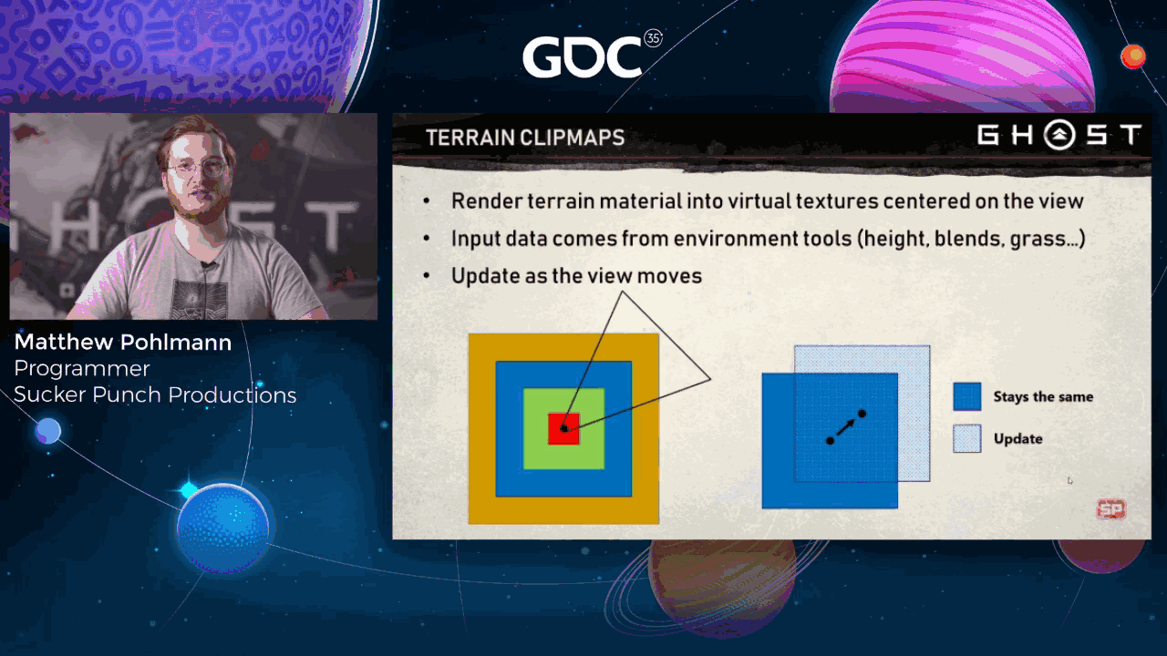
Terrain clip maps aren’t exactly a new concept, but they’ve worked very well for us. Rather than rendering terrain materials from scratch in pixel space every frame, we render terrain materials into an array of 2D textures. When drawing the actual terrain geometry, all we have to do is sample these pre-rendered textures, which avoids a lot of pixel shader cost.

We ship with roughly eight layers, where each layer is the same texture resolution but covers a larger area of the world. When rendering a pixel of the terrain, we choose which layer to sample based on the pixel’s distance from the camera. These 2D textures are updated as the view moves along the terrain.

Rather than shifting the contents of the entire texture, we shift a virtual center point. The majority of texture stays the same frame to frame, and instead, we only have to update strips along the edges. When sampling, we shift our sample point by the center point offset and use a wrapped sampling mode.

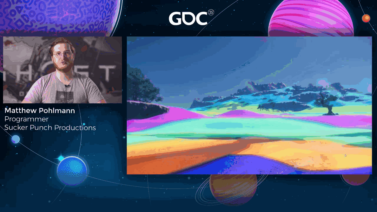
Here’s a short clip of visualizing clip maps in the engine. Note that the clip maps are axis-aligned in world space and they don’t rotate with the camera. Also, because the view is slightly at eye height, it’s usually at eye height. We actually push the center of the clip maps out in front of the camera a bit, so the highest resolution textures end up more central.

Slide 40 — 00:30:06

📌 要点汇总

地形像素在剪贴图边缘会混合当前剪贴图和更大剪贴图的贡献，以实现更平滑的过渡
这种混合技术有助于减少地形接缝处的视觉不连续性
剪贴图边缘的像素需要同时访问多个层级的地形数据

Terrain pixels on the outer edges of clip maps end up blending some contribution of that clip map and the next larger clip map for smoother transitions.

Slide 41 — 00:30:14

📌 要点汇总

每帧仅更新一到两个clip map层级以节省GPU时间
快速移动视角时优先更新高细节层级以保持画面清晰
相机切换时从第二层级开始更新，避免过近地面的渲染问题
特殊镜头（如近距离列车）优先更新层级0和1
静止视角时采用轮询方式更新所有clip map以确保地形贴图完整显示

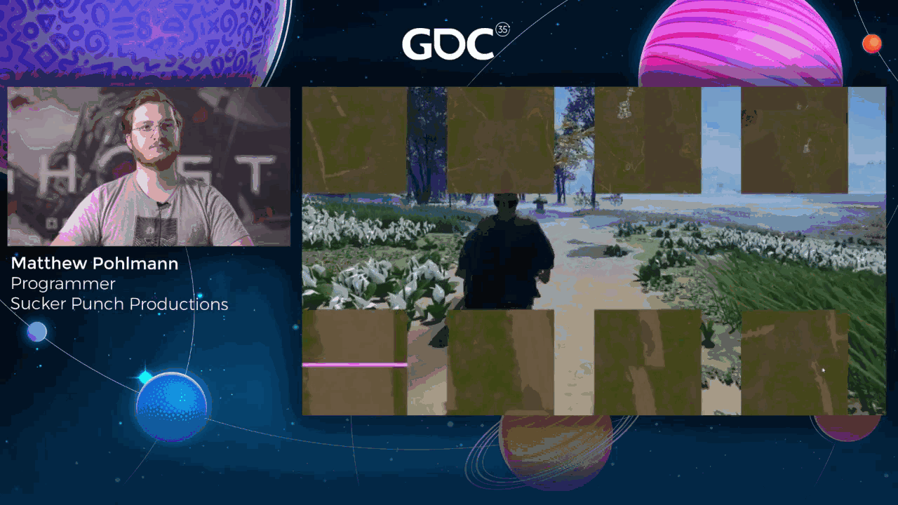
We usually only update one or two clip map levels per frame to save GPU time, so each frame updates a different set of clip map levels until they’re all up to date. Because not all clip map regions are valid all the time, sampling may require falling back to larger clip map layers with lower detail. If the view is moving quickly, we bias our updates towards higher levels to keep up and skip some updates on smaller levels, which are likely blurry on screen anyway if the camera is moving quickly.

On camera cuts, we dirty all clip map levels but start updating at layer two rather than zero, in the hopes that the camera isn’t too close to the ground. Though we did add a special close-up terrain camera feature to handle specific cuts like this, where the camera is very close to the train, where we update level zero and one first instead.

We also do a round-robin update of all clip maps when the view is stationary to catch terrain decals that are slow to stream in. Otherwise, you might have a decal rendered into one clip map level and not another, or missing entirely. This isn’t the greatest solution, but it was easy, and you generally never notice that this is happening.

Slide 42 — 00:31:13

📌 要点汇总

使用地形混合、湿润度、水洼和草地地图作为渲染剪贴图的输入
剪贴图着色器将材质数组中的数据混合在一起
当剪贴图区域失效时，生成重叠的地形贴图并进行二次渲染
在像素着色器中采样剪贴图，避免昂贵的材质混合计算

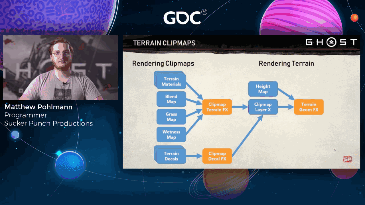
Rendering a clip map takes as input the terrain blend, wetness, puddle, and grass maps from the environment tools, and a list of terrain material definitions containing material textures and properties. The splat maps index into the material array, and all this data gets blended together in a special rendered clip map shader. When a clip map region is invalidated, we also generate a list of overlapping terrain decals and render them to the clip maps in a second pass. When we go to render our actual terrain geometry within the clip map, we sample these clip maps in the pixel shader, rather than doing any expensive material blending.

Slide 43 — 00:31:47

📌 要点汇总

PS4 Pro 上渲染场景时，不使用 clip maps 会导致火车绘制耗时 12 毫秒，占 33 毫秒预算的大部分
使用 clip maps 可显著节省 GPU 时间
静止状态的开销来自之前提到的 round robin 更新机制
跑步状态的开销是因为视图在移动，每帧需更新每个 clip map 的条带

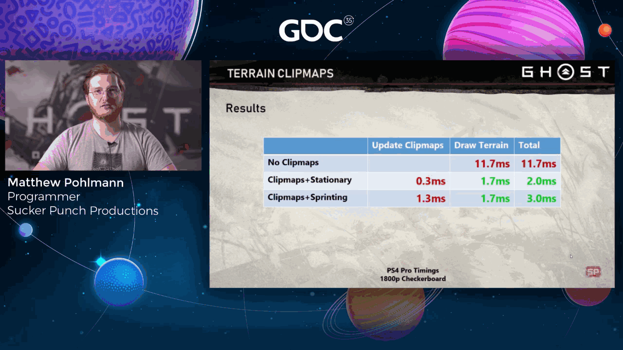
Here are some representative numbers taken on a PS4 Pro. When rendering this scene without using clip maps, drawing the train takes almost 12 milliseconds of our 33-millisecond budget. As you can see, clip maps save a huge amount of GPU time.

Note that the stationary cost comes from our round robin update that I mentioned earlier, whereas the sprinting numbers are because the view is actively moving and we’re updating strips of each clip map every frame.

Slide 44 — 00:32:11

📌 要点汇总

地形渲染成本高是因为每个 texel 可能受三个 alpha 权重材料影响
使用特殊混合函数结合 texel alpha 和每材料高度图进行混合
单个 clip map texel 可能需要混合最多 12 个材料
在着色器中通过标量循环处理最多 12 个材料 ID 和权重
标量化减少寄存器压力并避免纹理采样发散
实际中每个像素通常只混合 1-2 个材料，最多不超过 4 个

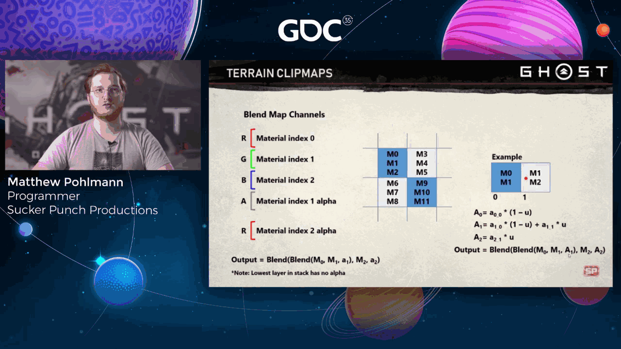
Part of the reason rendering our terrain is so expensive is because of the complexity of our terrain material blending. Each terrain texel can be influenced by three alpha-weighted materials, which is then blended over the previous using a special blend function that takes into account both the texel’s alpha and a per-material height map used for blending. Of course, we want blends to be smooth between texels, so in reality, a single clip map texel might have to blend up to 12 materials because of a bilinear blend of four neighbors in the flat maps, and all neighbors having three unique materials.

To accomplish this, we gather the up to twelve material IDs and blend weights required by the current pixel, then iterate over them in a scalarized loop in the shader by increasing material ID. Scalarization reduces register pressure in the shader and is required anyway so that we don’t have divergent texture samples. In most cases, a pixel will only iterate once or twice, but there are places where there’ll be three to four materials to blend. We very rarely have to blend more than four materials in practice.

Slide 45 — 00:33:10

📌 要点汇总

使用宏实现混合代码的标量化解，通过采样邻近 texel 并确定混合权重
s-compact 混合结构将 ID 和权重压缩为两个整数以节省寄存器
通过循环处理所有唯一材质 ID，每次迭代查找局部最小 ID 并与主线程 ID 比较
匹配时执行混合逻辑，否则线程在该迭代中处于休眠状态
完成一个 ID 处理后将其从压缩 ID 列表中移除，避免后续迭代重复处理

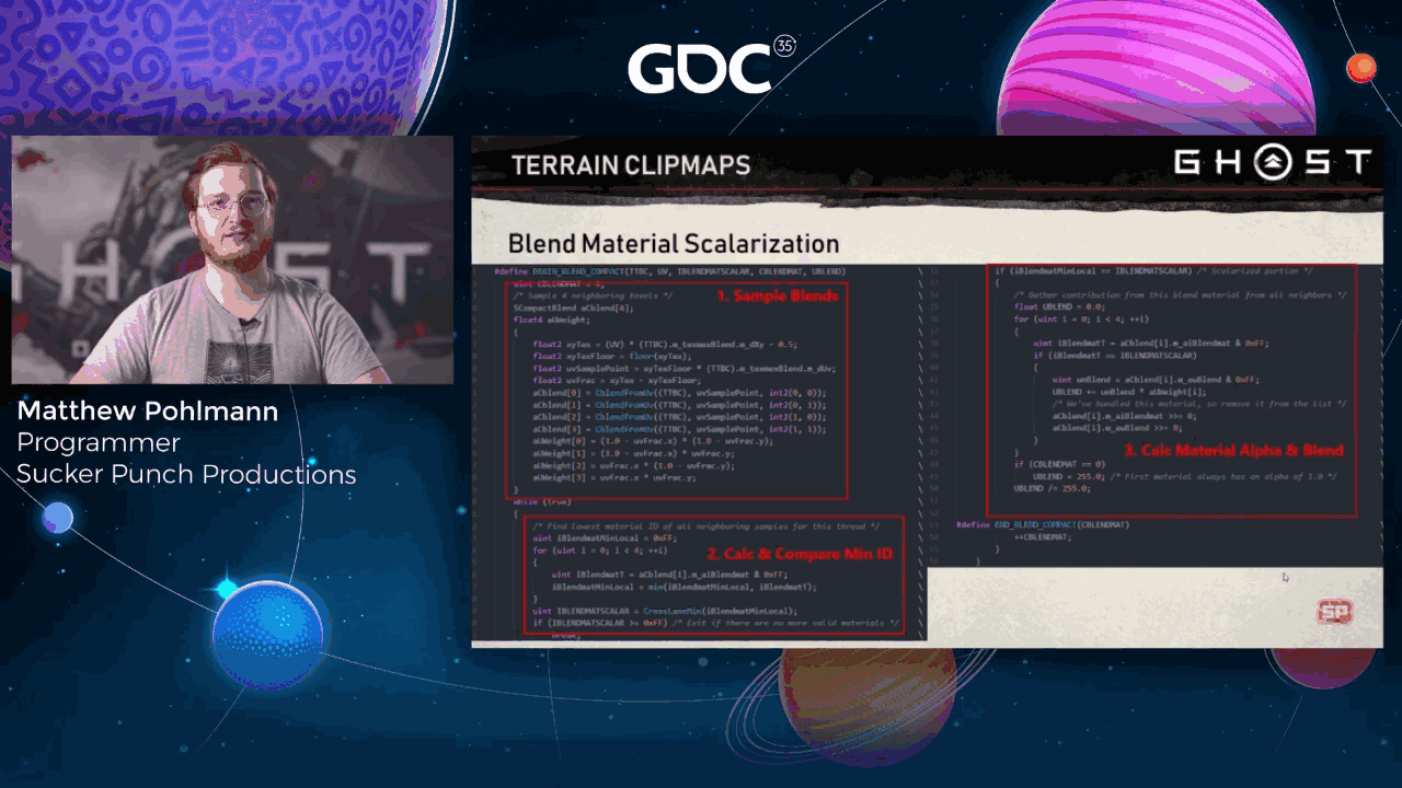
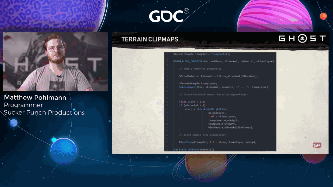
Here’s the somewhat gross macros we use to accomplish the scalarization of our blending code. Feel free to pause here if you want to browse the code; I’m not going to go into great detail. We first sample all neighboring texels and determine their blend weights. Note that the IDs and blend weights in the s-compact blend struct are compacted into two integers to save registers.

We then proceed into a loop that continues until we’ve exhausted all unique material IDs among our samples. And in each iteration, we find our local minimum ID and compare it to the main ID across all active threads. If we match, then we run our blending logic. Otherwise, we’ll be dormant for this iteration.

When we finish with an ID, we shift it off the end of our packed ID list so that it’s no longer considered for the next iteration.

Slide 46 — 00:33:53

📌 要点汇总

宏包裹在采样循环中，用于材质混合
阈值软度是每个材质的参数，控制与下方材质的混合程度

These macros get wrapped around our sampling loop, like so. There’s a bunch of other stuff I’ve removed for brevity, but this is the core of our material blending. The threshold softness input to the blend function is a per-material parameter that controls how softly it blends with materials below it in the stack.

Slide 47 — 00:34:09

📌 要点汇总

特殊的 alpha 和高度混合代码实现中，alpha 混合部分遵循标准 alpha 混合规则
混合顺序影响最终效果，高索引材质会覆盖低索引材质
该方法受到网上文章启发，并适配到支持多材质的着色器中

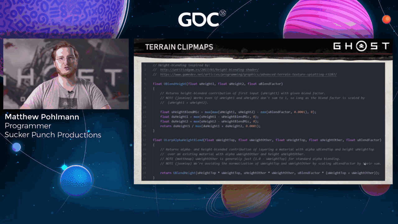
Here’s what our special alpha and height blending code looks like. Because the alpha portion of the blend is like standard alpha blending, the order we blend in matters. Materials with higher indices get blended over materials with lower indices.

You can see how we call this method on the previous slide. This dual alpha and height blending was inspired by some articles I found online and adapted to work in our shader with more than two materials.

Slide 48 — 00:34:31

📌 要点汇总

左侧为无材质高度混合的 alpha 混合效果，中心为 100% 岩石纹理，边缘为 0% 岩石
草地材质配置合适的混合因子并启用高度混合后，过渡更自然，细节更丰富
混合因子影响材质过渡效果，岩石使用低因子（锐利过渡），沙地使用高因子（柔和过渡）
实际场景中发现了多种自然美观的材质混合效果

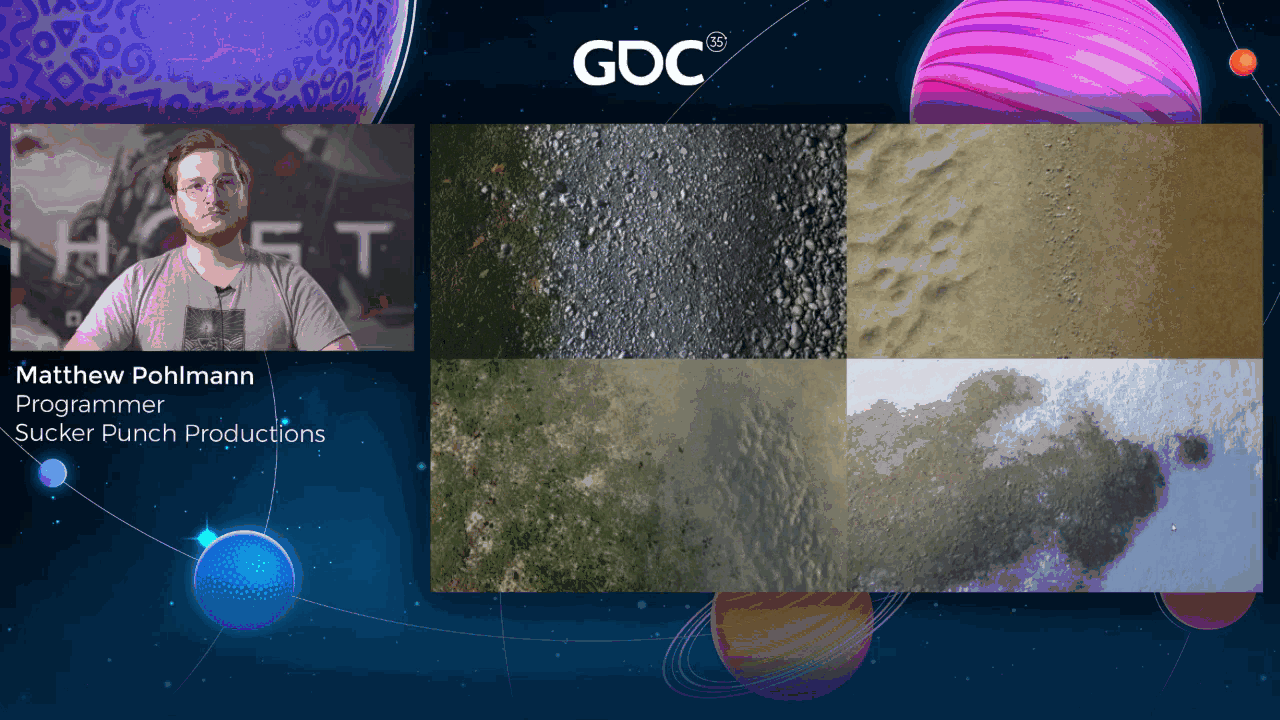
On the left is just alpha blending without per-material height blending. The center of the rocky texture is 100% rocky, then the 50/50 blend, and then 0% rocky as you reach the edge. This doesn’t look particularly amazing. When the grass material is configured with a decent blend factor, though, and I re-enable height blending, then it looks like the image on the right. The blend looks a lot more natural and less smudgy, and we get interesting micro details from the height maps in the transition area between the two materials.

Here’s what happens when I vary the blend factor from 0.001 to 0.5 of that top grassy texture. Different materials are configured with different factors. For example, a rocky texture will use a low blend factor, so it has sharp cutoffs, whereas something like sand will have a higher blend factor, so it has softer blends with materials below it.

Here’s a couple nice-looking blends that I found roaming around the world.

Slide 49 — 00:35:25

📌 要点汇总

地形材质中存在明显的拼接伪影
通过将 texels 分配给基于世界空间位置的 Voronoi 单元来避免伪影
每个瓷砖应用随机 2D 旋转以统一材质 UV 查找
单元边缘需要融合最多三个相邻单元的贡献以实现平滑过渡
启用 Voronoi 拼接后伪影显著减少

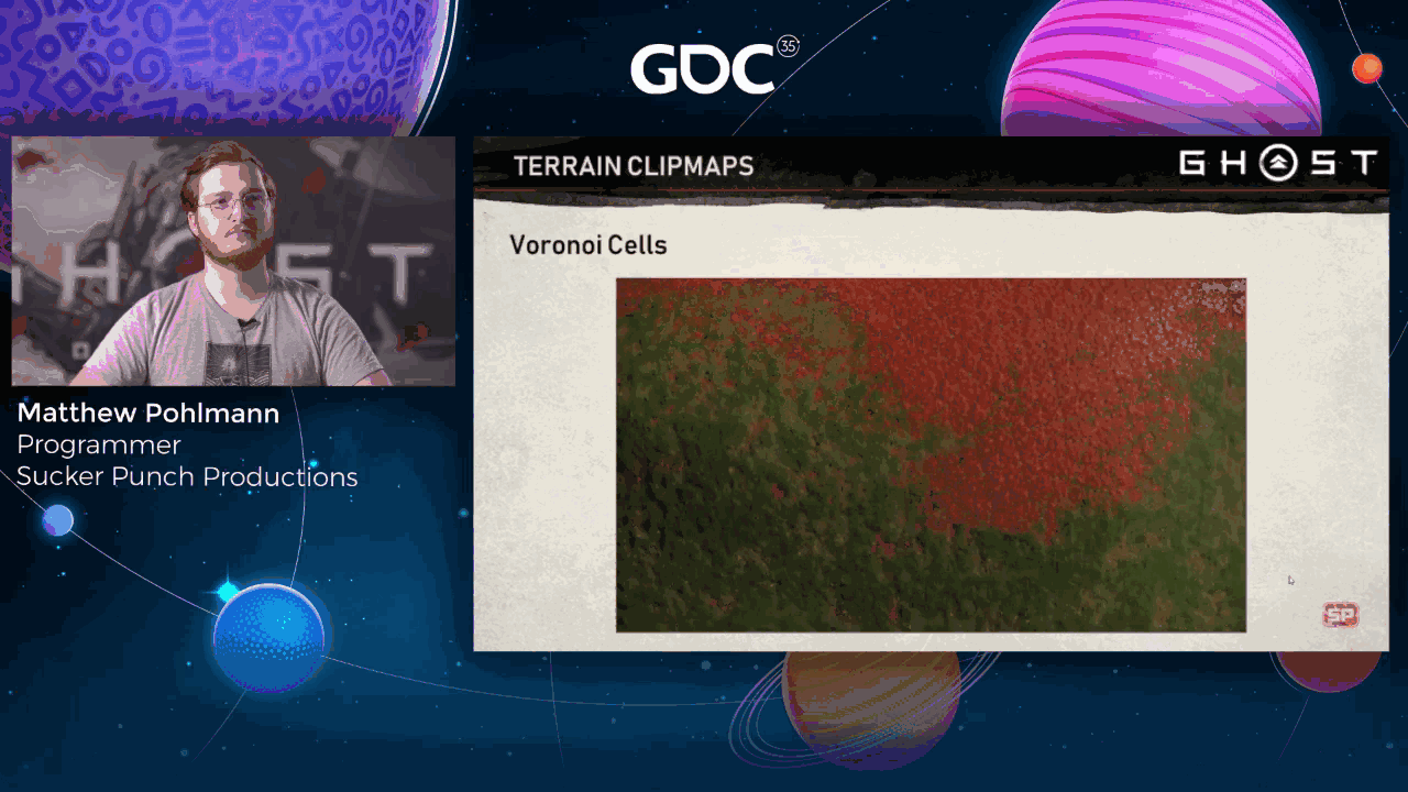
Here you can see some obvious tiling artifacts in our terrain materials. To avoid this, we assign texels to Voronoi cells based on their world space position. Each tile gets assigned a random 2D rotation to apply to all material UV lookups, and the edges of cells have to blend contributions from up to three neighboring cells for smooth transitions.

Here’s the same shot from before with no Voronoi tiling. Here it is with Voronoi tiling enabled.

Slide 50 — 00:35:58

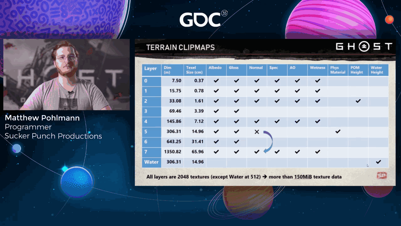
📌 要点汇总

CLIMAP 层包含 albedo 和 gloss 通道，部分层如层三跳过其他通道
层五包含 CPU 可访问的物理材质图，用于采样附近地形类型（如泥泞、沙地、岩石）
层二包含高分辨率细节高度图，用于地形视差遮挡映射
存在独立的低分辨率水高度图，用于动态湿润效果
渲染时若某层缺少通道，将回退到包含所需值的下一层
除水高度图外，所有 CLIMAP 纹理为 2K 分辨率，总大小略超 150MB

Here’s the makeup of all of our CLIMAP layers. All standard layers have albedo and gloss, but other channels are skipped for partial layers like layer three. There are also a couple of special layers and channels used by various runtime systems. Layer five includes a CPU-accessible physics material map for sampling nearby terrain phys types, like whether it’s muddy or sandy or rocky. Layer two has a high-res detail height map used for terrain parallax occlusion mapping. And there’s a separate low-res water height map used by some geometry to opt into becoming dynamically wet-looking when near water.

If we sample a missing channel from our chosen clump map layer when rendering, we instead fall back to the next larger layer that contains the value we need. For example, if we want the normal at layer five, we’ll get it from layer seven instead. All clump map textures are 2K except for the water height texture, so altogether they take up just over 150 megabytes.

Slide 51 — 00:36:54

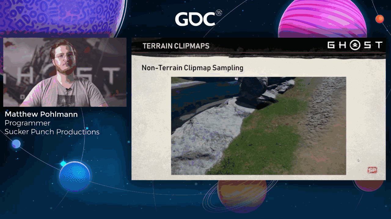
📌 要点汇总

远距离未被clip maps覆盖的地形使用简单的漫反射材质
该材质通常被植被、阴影或雾气遮挡，视觉影响较小
跌回路径使用与之前相同的标量混合宏，但简化了内循环
不使用地形贴图来渲染道路，避免在远处消失的问题
使用地形表达式替代道路贴图，使道路渲染更高效且延伸至远处
非地形着色器可选择采样clip maps以实现更自然的材质和法线混合
艺术家可通过顶点绘制控制每种资产的混合区域

For faraway terrain that isn’t covered by clip maps, we fall back to a simple diffuse-only non-visual terrain material. The image here, that’s everything outside of the blue-tinted terrain. This doesn’t look amazing, but it’s generally not noticeable since faraway terrain is usually hidden by vegetation, shadows, or fog. You’ll note that not much actual terrain is visible in the distance here in these screenshots.

This fallback path uses the same scalarized blending macros as before, but the inner loop is simplified. Only sample material albedo. One interesting thing of note is that we don’t use terrain decals for our roads. That was our initial implementation, but because our clip maps don’t cover the entire island and the fallback doesn’t include decals, roads would disappear in the distance. Luckily, our terrain blending materials saved the day.

We replaced all of our road decals with terrain expressions that output road-like materials along our road splines, and now our roads render off into the distance and are also cheaper. Non-terrain shaders can optionally sample clip maps to provide more pleasing material and normal blending with the terrain. Artists can control where blending occurs per asset by vertex painting.

Slide 52 — 00:38:04

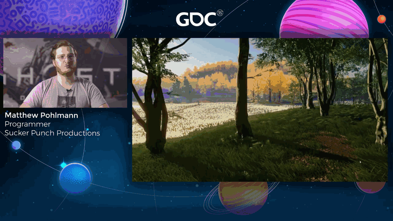
📌 要点汇总

Proxy sets 是 Ghost 中用于处理极高实例数量对象的 GPU 计算版本的实例化技术
几乎所有植被和其他资产都使用了 proxy sets 进行渲染
剩余植被可能是手动放置或实例数量较低，因此使用传统方法渲染

Next, I’ll walk you through a rendering feature we call proxy sets—a GPU compute version of instancing we created for Ghost. Proxy sets are a special rendering code path that we added to handle very high instance count objects. In these images, almost all the vegetation and many other assets are proxy sets. Remaining vegetation might be either manually placed, or the instance count of that particular asset was low enough that we rendered it with traditional methods instead.

Slide 53 — 00:38:33

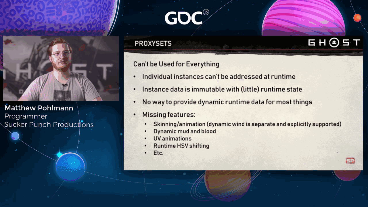
📌 要点汇总

使用代理集（proxy sets）减少每个实例的内存和CPU开销
代理集将剔除（culling）工作转移到GPU，提高性能
代理集用于相同资产的多个实例，如树木、灌木等
代理集不支持对单个实例进行动态控制或修改
代理集不替代现有实例渲染路径，仅用于高实例数量的资产
支持每个实例的LOD渐变状态（stipple fade state）字节数据

We quickly realized that with the sheer number of objects in the environment, we were going to break our memory and CPU budgets very quickly. Proxy sets were designed to attempt to solve both of these issues by reducing per-instance allocations and moving culling work to the GPU. A proxy set is essentially a group of instances of the same asset, like a particular tree or bush. Each instance is mostly identical, and any varying data is highly compressed and as minimal as possible. Surviving instances get drawn via instance draw calls. In Ghost, most environment assets are drawn via this code path. This includes trees, bushes, flowers, and rocks. Though some high instance count man-made objects are also included, like fence planks or castle pieces. Note that this does not replace our existing instance rendering code path, but is used instead for assets with very high instance counts.

Proxy sets are designed to be as efficient as possible and don’t provide a way to address individual instances. Their data is mostly immutable, and the runtime has no way to provide per-instance dynamic state. Because of this, proxy sets aren’t as fully featured as our traditional rendering pipeline, though this is generally fine, as environment assets usually don’t use any of these unsupported features anyway. The main piece of per-instance data that we do support at runtime is a byte tracking per LOD stipple fade state. When an object is transitioning between two LODs, we have to track how faded this particular LOD on that particular asset is.

Slide 54 — 00:39:52

📌 要点汇总

展示了编辑器中的力反馈日志过渡效果
该功能同时支持传统渲染管线和代理集
每一帧都会更新淡入淡出的字节数据

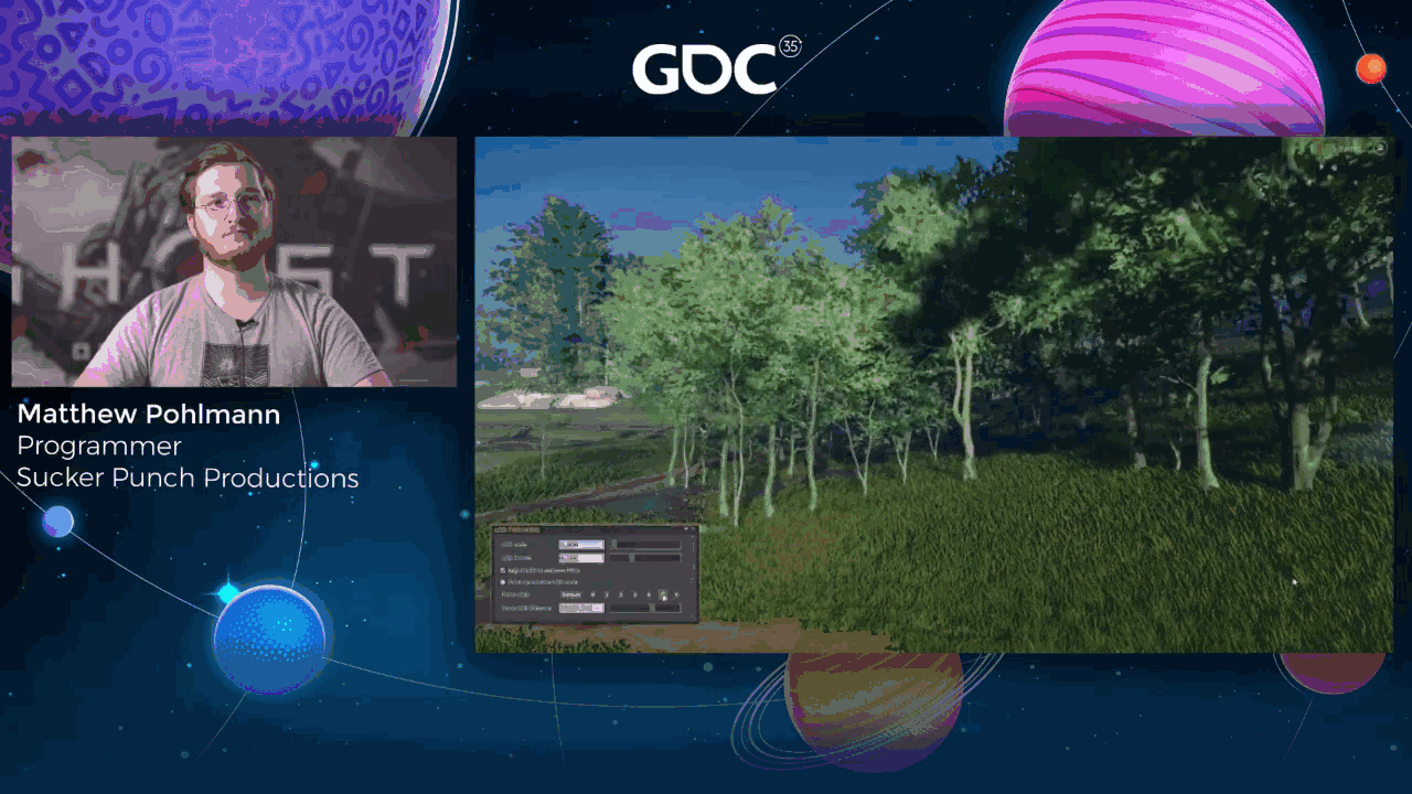
Here’s a quick video showing a force log transition in the editor. Note that this feature is supported by both our traditional rendering pipeline and proxy sets, and these fade bytes get updated every frame.

Slide 55 — 00:40:07

📌 要点汇总

每个实例使用24字节存储旋转和缩放信息，通过单个uint打包
精确模式使用40字节，适用于需要高精度对齐的资产（如城墙、围栏）
代理集相比传统方式显著减少内存占用，从n×s降至n+s
高实例数量的地形瓦片内存占用减少高达70%

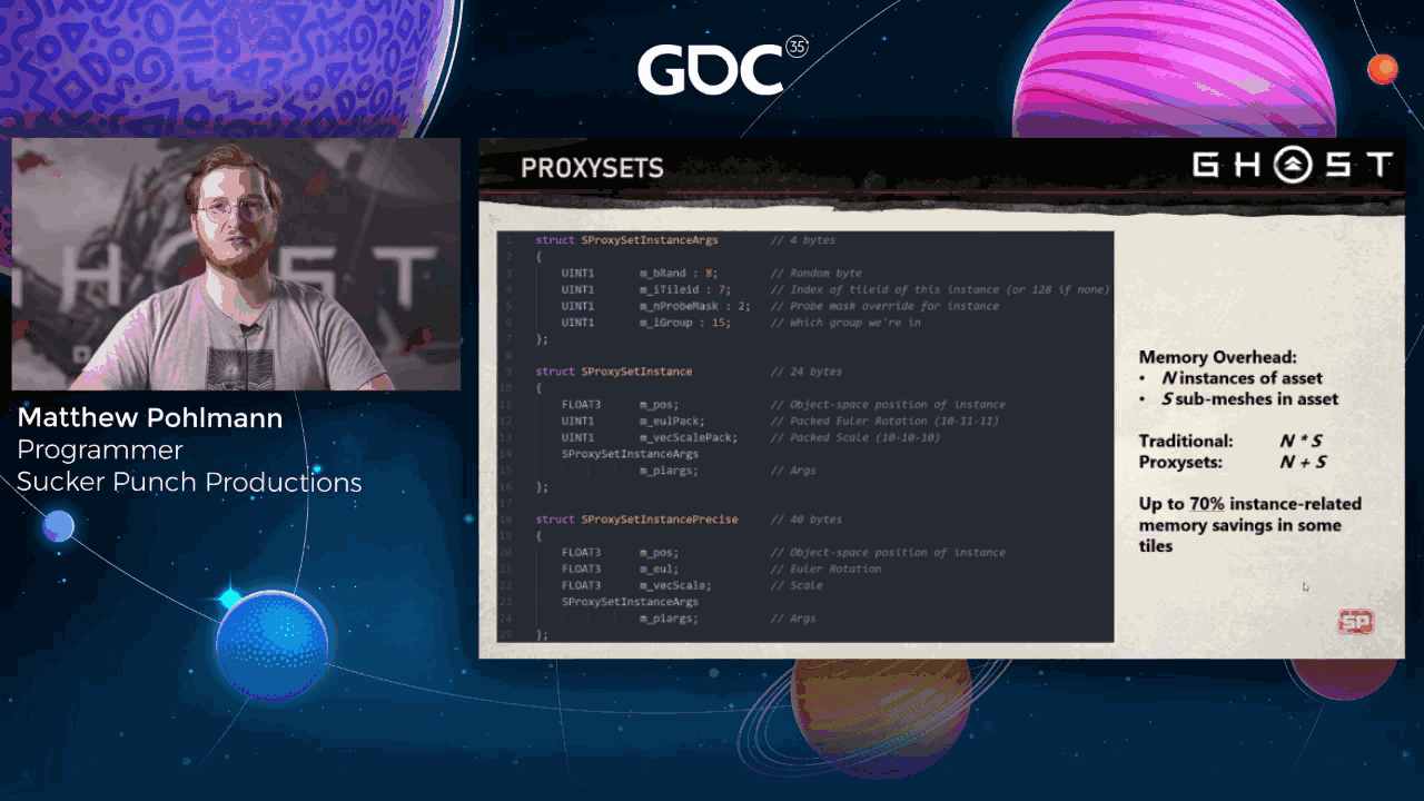
The vast majority of proxy sets use a 24-byte per instance setup, where three component rotation and scale are each packed into a single uint and unpacked when needed. The 40-byte precise variant is an option for specific assets that need additional precision for rotation or scale, and is mainly useful for things that need to line up perfectly, like castle wall segments or fence boards.

This setup saves a lot of memory compared to our traditional path. Whereas before, if we had n instances of an asset with s submeshes, we’d end up with memory overhead on the order of n times s. Proxy sets lower this to n plus s via extra indirection and simplified instance data.

It’s a little hard to quantify due to how deeply integrated proxy sets are, but I estimate that some terrain tiles with high instance counts saw up to 70% reduction in drawable instance-related memory.

Slide 56 — 00:40:54

📌 要点汇总

支持随机实例脱落（stochastic instance fall-off）功能，用于优化远处网格的细节层次（LOD）
实例脱落是基于构建时生成的每个实例的随机字节输出，具有确定性
实例脱落速度可根据资产进行配置，提升性能和视觉效果平衡

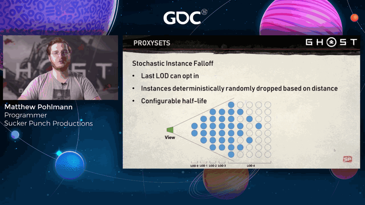
Practices support a feature called stochastic instance fall-off, where the final LOD of a mesh can opt into having instances randomly dropped as they get further from the camera. This randomness is deterministic and based on a per-instance random byte output at build time. How quickly instances are dropped is configurable per asset.

Slide 57 — 00:41:12

📌 要点汇总

未启用随机衰减时，远处岛屿末端的森林非常密集，绘制约100,000个代理实例
启用随机衰减后，远处森林变得稀疏，节省约50,000个绘制实例
每次节省约1.17毫秒GPU时间
这种优化在游戏中的高点和清晰天气下才可见，远处缺失内容难以察觉

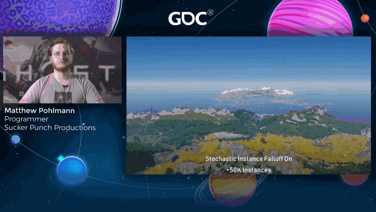
Here’s what an overview of Sushma looks like without stochastic fall-off. Note specifically the dense forest off in the far distance on the very end of the island. Here we’re drawing roughly 100,000 proxy set instances. And here we are with the feature enabled. Note the much sparser forest in the far distance, and that we’ve saved about 50,000 instances of drawing. This equates to roughly 1.17 milliseconds saved on the GPU.

It’s rare to ever have a view like this in the game, even at the highest point on the island with the clearest weather. So it’s pretty tough to notice that things so far away might be missing.

Slide 58 — 00:41:52

📌 要点汇总

使用 CPU 进行粗略剔除，一次性丢弃数千个实例
剩余代理集通过异步计算管道在 GPU 上处理
GPU 通过视锥体和包含缓冲区进行剔除，与前一帧图形工作重叠
GPU 使用小着色器分配实例流内存，避免间接绘制
初始方案使用 GPU 异步模型和间接绘制，导致大量空绘制
跳过 2,000 个空绘制可节省 0.67ms GPU 和 1.5ms CPU 时间
GPU 节省主要来自不处理空的间接绘制
下一帧运行构建流着色器，将稀疏数组压缩为密集实例流
构建流和实例绘制用于最终渲染，显著优化性能

Here’s an overview of what a proxy set frame looks like. Once the main game update is done, we know what objects want to be rendered. We do a very coarse culling pass of all proxy sets and the entire proxy set level on the CPU, which lets us throw out thousands of more or more instances at once. Surviving proxy sets are then dispatched to an async compute pipe on the GPU. The GPU calls all of these instances against the view frustum and inclusion buffer for the main view in a high-priority async compute pipe. Note that this overlaps graphics work from the previous frame on the GPU.

Once the final instance counts are known, the GPU runs a tiny shader to allocate per-instance instance stream memory out of a linear allocator. The CPU syncs against the async GPU compute work once instance counts are known and memory has been allocated, and then records standard instance draws because we now actually know the instance counts. We don’t need to do indirect draws. This part was actually very important for us. Our initial implementation used a fully GPU async model and instanced indirect draws, but that meant we had to submit draws for proxy sets with zero surviving instances after calling.

In some scenes, skipping over 2,000 empty draws meant saving up to 0.67 milliseconds on the GPU and one and a half milliseconds on the CPU. Surprisingly, most of the GPU savings actually came from the GPU not having to process empty instance indirect draws. At the beginning of the next GPU frame on the graphics pipe, we run the build stream shader, which is responsible for compacting the sparse arrays of surviving instances down to densely packed instance data streams containing data like the object-to-world matrices and whatever else we need for instance rendering draws.

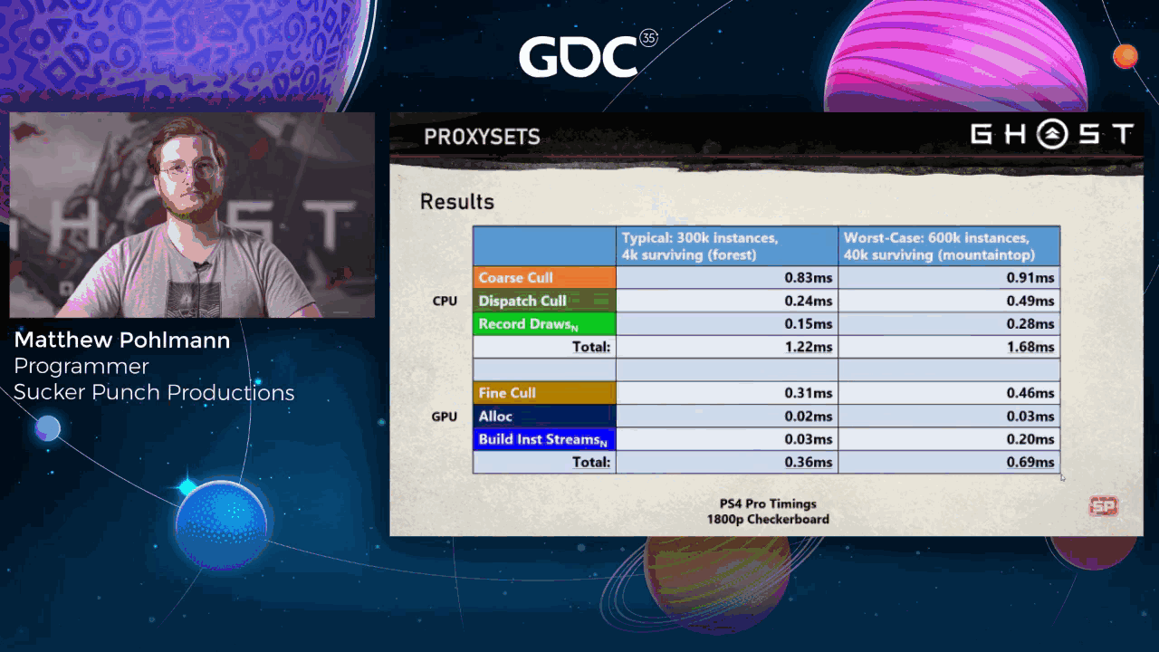
The built streams and instance draws are then used to render everything. Here are some results showing both CPU and GPU costs for the various stages from the previous slide.

Slide 59 — 00:43:44

📌 要点汇总

使用实际渲染场景的深度数据进行遮挡剔除检查
检查必须保守，避免误判遮挡情况
生成前一帧深度缓冲区的 mip 链，起始分辨率为四分之一
每个 mip 使用最大值滤波而非线性混合
对物体进行测试以判断是否被遮挡

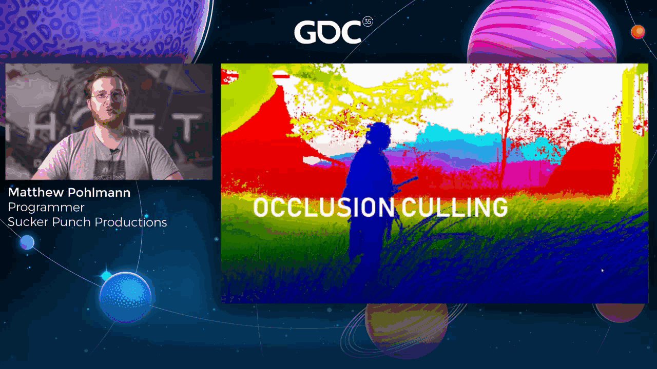
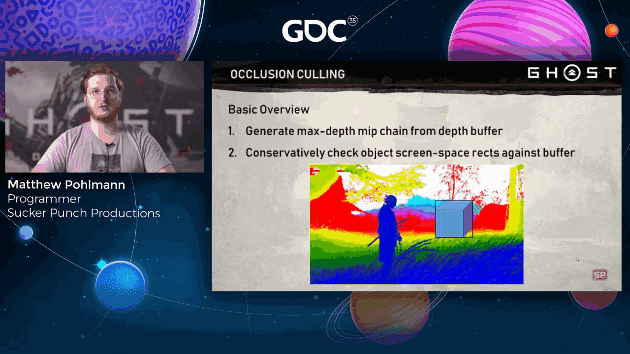
Next, I’ll describe our approach to depth-based occlusion culling. The basic idea is that you use depth data from your actual rendered scene as a way to check whether an object might be occluded or not. These checks have to be conservative, so you don’t accidentally occlude something, and we want them to be fast. So we generate a mip chain of the previous frame’s depth buffer starting at quarter resolution. Each mip uses a max filter rather than a linear blend. And testing an object.

Slide 60 — 00:44:15

📌 要点汇总

计算缓冲区的屏幕空间边界矩形以判断遮挡
测试矩形内所有重叠像素的深度值与物体最近深度值进行对比
仅当物体最近深度值在矩形内所有像素之后时，才判定为被遮挡

Against this buffer involves calculating its screen space bounding rectangle and testing all overlapping occlusion depth pixels against the object’s nearest depth value. Only if the nearest depth of the object is behind all occlusion buffer pixels in that rectangle can you say that it’s occluded.

Slide 61 — 00:44:30

📌 要点汇总

CPU 仅访问纹理的 mip zero 层，通过 SIMD 代码每次加载并测试四个 texel，实现快速 occlusion query
GPU 使用所有 mip 层进行 proxy set 渲染，从最高 mip 开始采样，最多 64 次采样
高 mip 层可快速 occlude 大量物体，部分物体需要低 mip 层的高分辨率信息
计算精确 mip 级别以覆盖物体屏幕矩形的方法虽使 occlusion 成为常数时间操作，但导致过多物体未被正确 occlude
初期 occlusion buffer 实现因使用前一帧深度缓冲导致 occlusion disocclusion 艺术效果，出现物体闪烁问题

In our implementation, the CPU has access to only mip zero of this texture for occlusion queries via a highly optimized SIMD code that loads and tests four texels at a time. This turned out to be fast enough for us, and since we’re using mip zero, we’re able to successfully occlude lots of objects. The GPU uses all available mips for proxy set rendering, starting at the highest mip. We sample until we’ve either decided that the object is occluded, we’ve run out of mips, or the number of samples for the current mip would exceed a threshold, which is currently 64 samples. Many objects get occluded with few samples at high mip levels, but some require the extra information in higher res mips. This ended up being a net win. The extra samples are generally cheaper than failing to occlude something that we otherwise could have skipped.

An alternative that we tried but ended up not using is to calculate the exact mip level required where two by two texels fully cover the object’s screen rectangle. This makes occlusion a constant time operation. Do some math to determine the mip level and then compare against exactly four texel values. In our case, this failed to occlude too many objects, so even though occlusion queries became much cheaper, we ended up drawing lots of hidden objects.

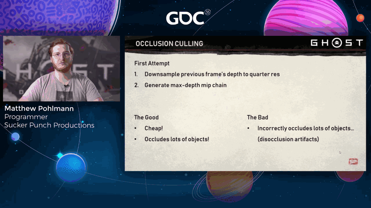
Our first attempt at implementing an occlusion buffer didn’t work out very well. It was simple and relatively cheap, and all we did was take the previous frame’s depth buffer as is and create a max depth mip chain of it starting at quarter resolution. The results seemed promising. We were able to occlude lots of objects and gain some significant performance wins, but then we started to get bug reports about objects flickering on screen, especially when the camera was moving quickly. This was occluded disocclusion artifacts. Objects were being reported as occluded when they shouldn’t be because the depth from the previous frame was not a good approximation of this frame’s depth.

Slide 62 — 00:46:14

📌 要点汇总

屏幕右侧在相机移动经过树木时出现闪烁现象
隐藏在树木后的物体在下一帧仍不渲染
原因是树木后方仅显示空的天空盒（skybox）
该问题属于视差遮挡（disocclusion）伪影的一种

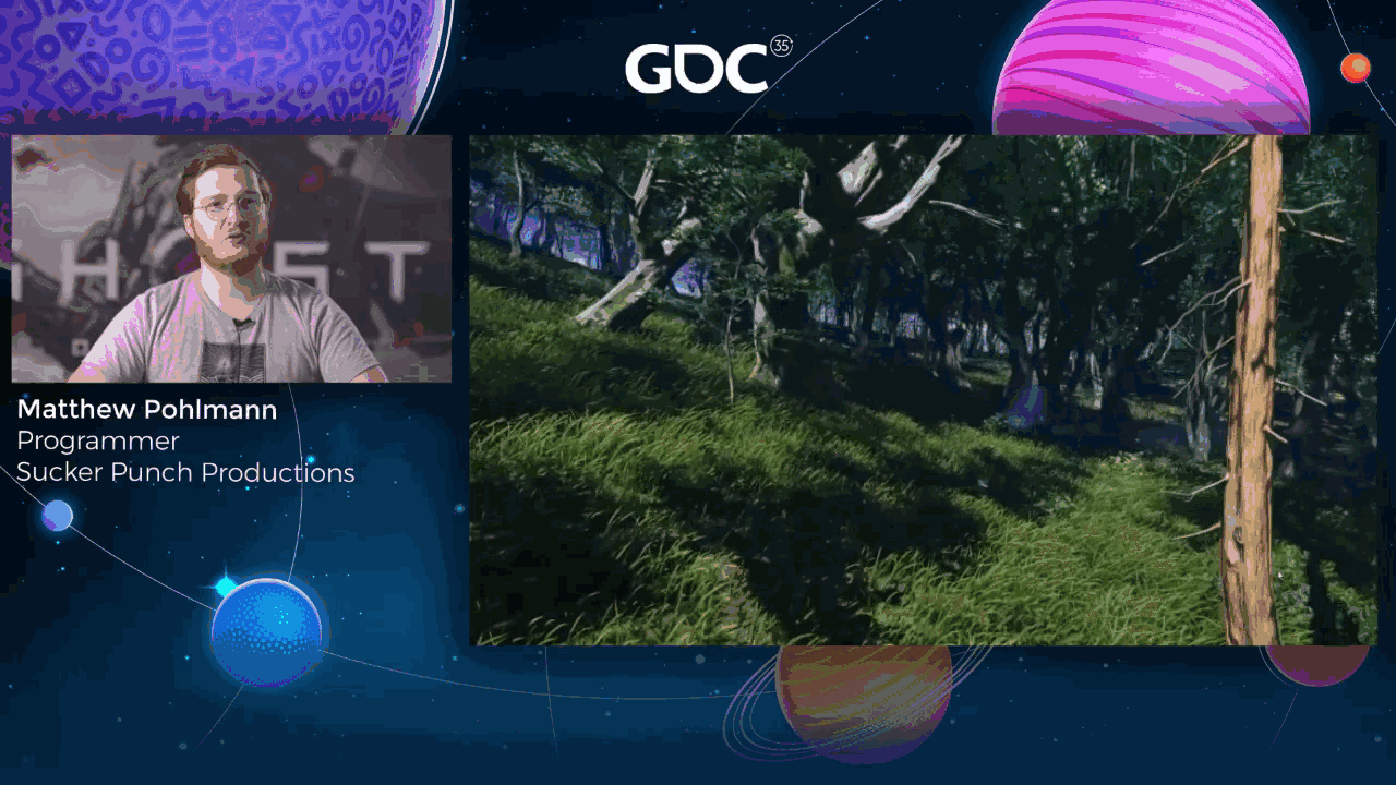
Here’s a video showing the disocclusion artifacts that I mentioned. Note primarily the flashes on the right-hand side of the screen as the camera moves past these trees. Objects that were previously hidden by the tree continue to not render for one additional frame, because all that’s behind them is an empty skybox.

Slide 63 — 00:46:33

📌 要点汇总

第二次尝试将前一帧的深度重新投影到当前帧的相机空间中
重新投影后出现深度信息缺失的“洞”，用远平面深度值填充
该方法消除了遮挡伪影，但填充效果不理想
使用最大深度链并填充远平面值，导致多数区域迅速变为远平面值
遮挡缓冲区设置为远平面，导致多数物体未被遮挡，浪费计算资源

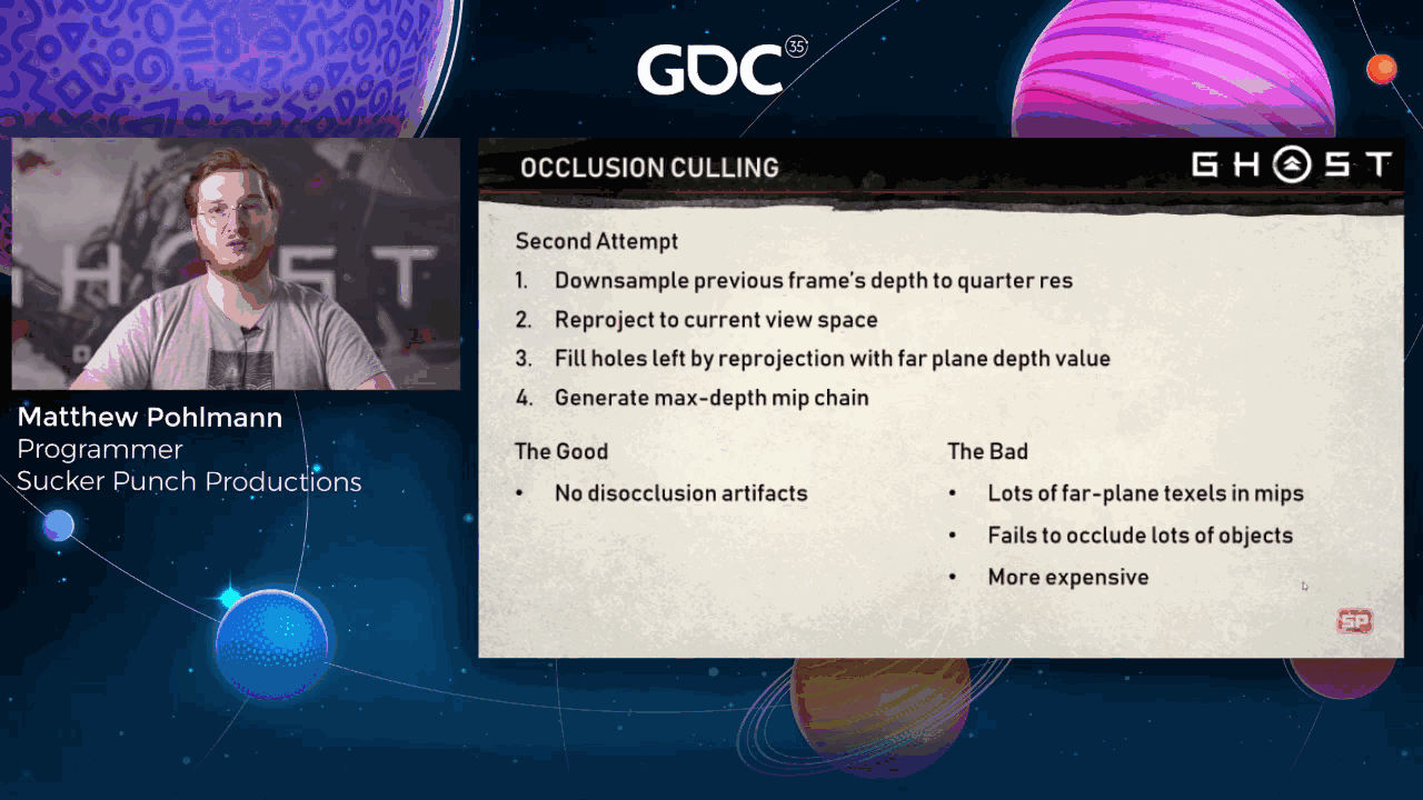
Our second attempt involved reprojecting the previous frame’s depth into the current frame’s camera space. This leaves behind holes where we don’t have any depth information after the reprojection, and we just fill those with the far plane depth value. This approach removed all disocclusion artifacts, but the hole filling was far from optimal. In fact, because we use a max depth chain and we were filling holes with the far plane value, it didn’t take many mip levels for practically everything to have the far plane value.

The occlusion buffer was set to the far plane. Very few objects would get occluded, so we were paying the price to create the occlusion buffer and sample it for most things, just to say that they weren’t occluded.

Slide 64 — 00:47:12

📌 要点汇总

新的重投影代码导致远平面值（白色像素）在更高mip层级迅速泛滥
这严重影响了遮挡缓冲区的功能实现
需要优化重投影算法以减少远平面值的过度扩散

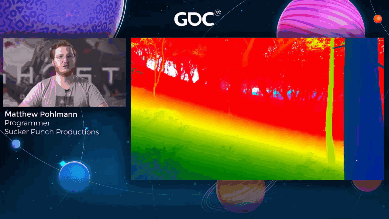
Here’s what the occlusion buffer looks like as I recreate that same camera motion as before, but with the new reprojection code. The white pixels you see are all far plane values, and as you can imagine, higher mip levels become completely flooded with white very quickly, which mostly defeats the purpose of the occlusion buffer.

Slide 65 — 00:47:31

📌 要点汇总

使用当前帧的极线点作为提示，在深度缓冲区中进行搜索以解决空洞填充问题
该技术通常用于从单张2D图像生成3D图像，通过第二视角重建深度和颜色数据
本研究仅需深度数据，并尝试重建未来时间点的数据，假设与前一帧足够接近
空洞填充成本增加，但能减少遮挡伪影并遮挡更多物体
极线几何中，右视图中的ER点对应左视图相机在当前帧屏幕空间中的前一帧相机位置
极线XR是左视图中点X在右视图空间中的投影线，X的深度不同会导致右视图中投影点不同

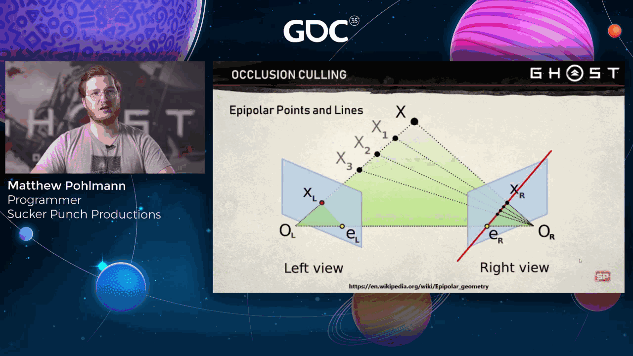
To solve the hole-filling problem, I did some research that led me down a hole of 3D image reconstruction techniques. The simplest one I found that seemed plausible to adapt involved using this frame’s epipolar point as a hint for performing a search in our depth buffer. Usually, this technique is used when you want to generate a 3D image from a single 2D image in stereoscopic rendering. The second eye uses the epipolar point to reconstruct depth and color data from a slightly different viewpoint, so you end up with two images: the original and the shifted one.

This technique works similarly for us, though we only need depth data, and we’re trying to reconstruct data at a future point in time as well. The hope is that things are still close enough to where they were on the previous frame that our depth reconstruction provides a good estimate. This makes hole filling more expensive, but we’re now able to occlude more objects with fewer disocclusion artifacts. Here’s the reference material I used when implementing our epipolar search, which I’ll explain in the next few slides.

Wikipedia probably does a better job than me of describing epipolar geometry, but here’s a brief summary. Here, the point ER on the right is an epipolar point. It is the location in the right-hand view space of the left view’s camera position OL. In our case, this maps to the previous frame’s camera position in the current frame’s screen space. The line ER to XR is an epipolar line. It’s a line segment describing the projection of the point X seen from the left. Put in the right view space. Note that from the left view’s perspective, X could be at any depth, one, two, or three, and depending upon where it actually is, you get a different point projected in the space of the right view. This is how we end up with a line.

Slide 66 — 00:49:13

📌 要点汇总

小圆圈表示关注的极点
上一帧相机位置投影到当前帧屏幕空间

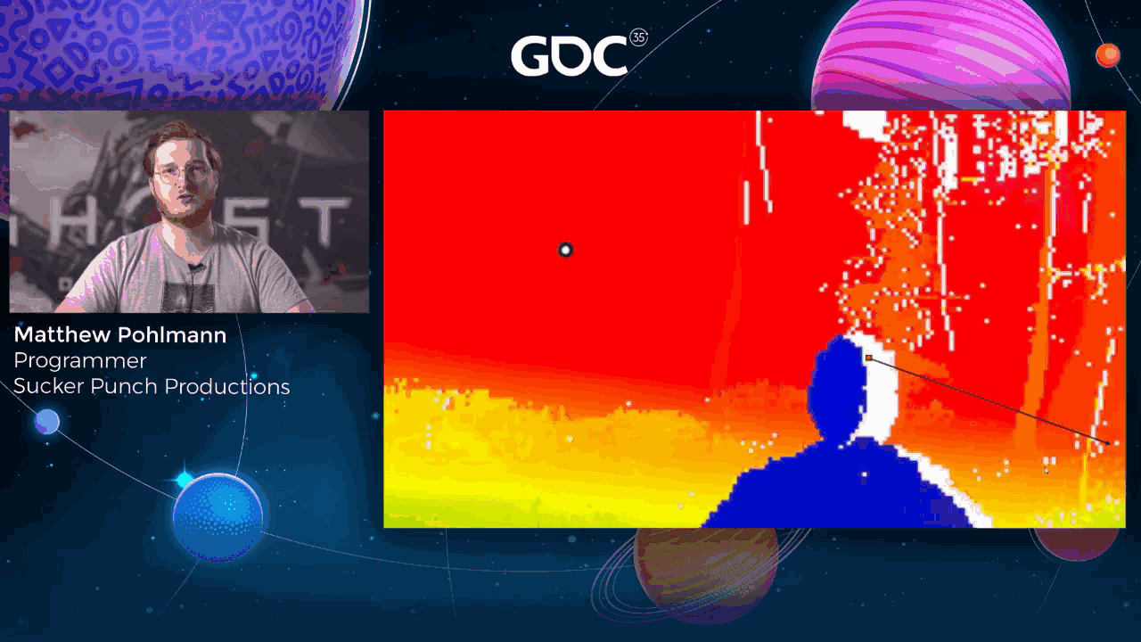
Here, the little moving circle is the epipolar point we care about. The last frame camera position is projected into this frame’s screen space.

Slide 67 — 00:49:23

📌 要点汇总

算法沿与极线相反方向搜索深度缓冲区，找到第一个有效深度值作为填充依据
绿色方块为中心像素，橙色像素为找到的深度值用于填充
空洞通常由前景几何移动导致，背景像素在前一帧无数据
搜索方向偏向背景几何，提高填充准确性
与前一帧深度值取最大值，增强保守性以解决凹凸前景问题
对于凹形空洞，前一帧沿极线的最大深度值通常足够有效

The hole-filling algorithm searches the depth buffer in lines opposite the epipolar point for each hole pixel. The first valid depth value we find is our approximate depth value. So here, the green square at the center of the image is the pixel I want to fill in. This is the line along which I will search. I find this kind of orangey depth pixel here, and I use that for my depth value.

The reason this works is because holes come about when foreground geometry has moved relative to the view, revealing background pixels that didn’t have data on the previous frame. The foreground geometry is always towards the epipolar point along a pixel’s epipolar line, so if we search in the opposite direction, we have a good shot at finding background geometry instead. We bias our search value a bit and take the max between this search value and the depth of this pixel on the previous frame to be extra conservative. This helps solve issues that arise due to.

Concave foreground geometry, like the hole between Jin’s arm and his body, in that case, searching in either direction along the epipolar line isn’t much help. But the max step along this line in the previous frame usually gives good enough results.

Slide 68 — 00:50:33

📌 要点汇总

演示了启用洞填充功能后的效果，远平面像素显著减少
远平面像素仅来自实际远平面和天空盒
填充区域（如 Jin 和附近树木边缘）出现模糊效果
填充功能有效减少了原本的洞区域

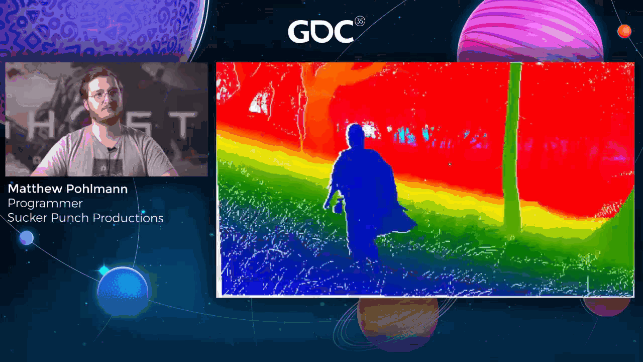
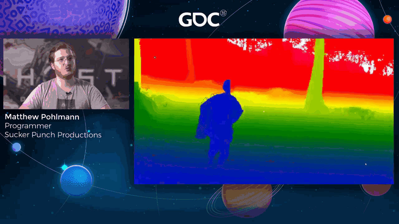
Here, I’ve tried to recreate that previous video I showed, but with hole filling active. Note that there are far fewer far plane pixels, and in fact, the only ones I could see are from the actual far plane and the skybox. You’ll also notice the somewhat smudgy appearance of the pixels along the trailing edge of Jin and the nearby trees, and these are areas where there previously were holes, but we’ve filled them.

Slide 69 — 00:50:58

📌 要点汇总

代码片段展示了深度重投影技术的实现
包含前向和后向投影两种操作
前向投影将上一帧的点投影到当前帧的新坐标
后向投影将当前帧远平面的点投影到上一帧用于深度采样
最终通过比较前向和后向投影结果取最大值

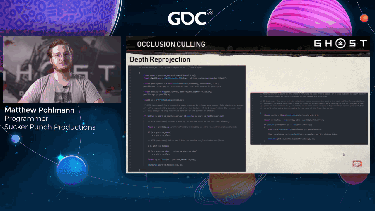
The next couple slides are a code dump of these techniques. I won’t go into great detail, but feel free to pause and inspect them more closely. Hopefully, the comments and variable names are enough to understand what’s going on. These code snippets are the main part of the depth reprojection code. Note that we do both a forward and backward projection. The former takes a point from the last frame and projects it into this frame at a new xy position. The latter projects a point on the far plane in this frame space to an xy point in the previous for a depth sample that we use. That we combine with the previous forward reprojection, and we take the max between the two.

Slide 70 — 00:51:34

📌 要点汇总

使用极线搜索进行空洞填充，避免逐像素线性搜索
通过逐步加倍步长和增加MIP层级来近似线性搜索
需要在空洞填充前生成MIP图
空洞填充前后需生成两次MIP图

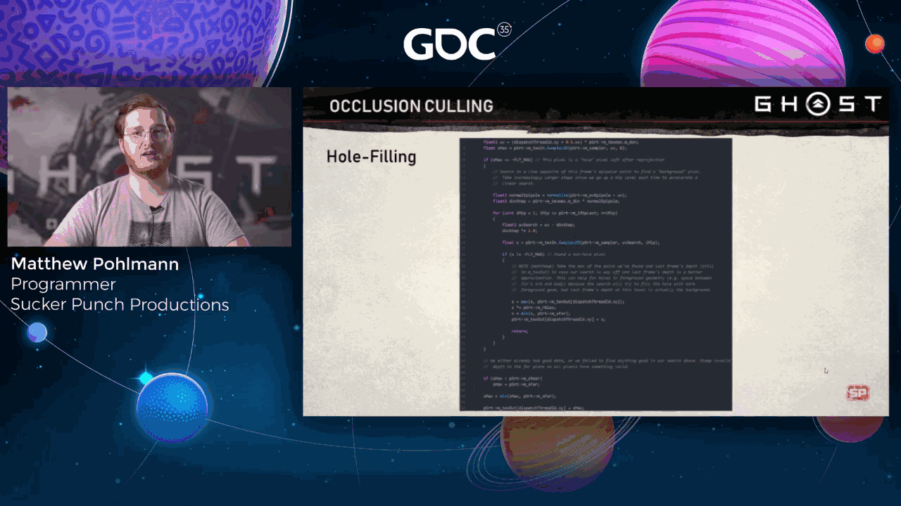
Here’s the core of the hole-filling algorithm using the epipolar search. Note that we don’t do a linear pixel-by-pixel search. Instead, we approximate a linear search by doubling our step size and increasing the mip level at each iteration. This requires that we’ve generated mips for a reprojected depth prior to hole-filling. So in reality, we have to generate mips twice: once prior to hole-filling, and then again after.

Slide 71 — 00:51:58

📌 要点汇总

异步计算管道显著降低遮挡缓冲区生成成本
绘制调用次数大幅减少，整体发送到 GPU 的数据更少
CPU 端可提前退出部分绘制设置和调度代码，节省资源
偶尔出现遮挡弹出现象，但整体发生频率较低
在 PS5 后向兼容模式下以 60 FPS 运行时，遮挡弹出现象更少

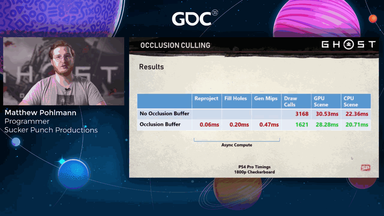
Here are the results from a short clip of me running through a forest. The occlusion buffer generation cost is mostly mitigated because we run it on an async compute pipe, but the vastly lower number of draw calls means we’re just sending way less to the GPU overall.

We’re also able to early out of a bunch of draw setup and dispatch code on the CPU, so we get big savings there as well. We still get the occasional disocclusion pop, but they’re pretty rare overall.

They’re even more rare when running the game at 60 FPS on a PS5 in backwards compatibility mode, since there’s less overall movement between each frame.

Slide 72 — 00:52:31

📌 要点汇总

计划对工具和运行时技术进行多项改进
重点提升性能和用户体验
未来将加强工具的可扩展性
持续优化运行时技术的稳定性

Lastly, I’d like to talk about some of the improvements we’d like to make in our tools and runtime tech going forward.

Slide 73 — 00:52:37

📌 要点汇总

快速迭代对获得良好结果至关重要，用户无法立即获取反馈和更改时，实验和优化意愿降低
提升表达编译速度和跨多帧增量评估表达式，可改善用户体验并加快实时预览反馈速度
当前600米热区范围尚可，但扩大范围将有助于整体森林场景的编辑和空间感知
希望实现世界级高度图编辑，并完全移除Maya和Flux工具以简化工作流程
在PlayStation硬件上实现这些功能需要创新，现有工具集虽好，但希望集成更多功能如道路、河流和悬崖编辑
当前生长资产碰撞问题可能不会解决，现有系统运行良好，但解决该问题会增加复杂性
当前遮挡缓冲算法表现良好，但仍偶尔出现遮挡突变，希望改进启发式算法使其更数学严谨
希望在地形表达式和绘制应用中增加更多图层，如海洋颜色和泡沫，以提升系统动态性和精度

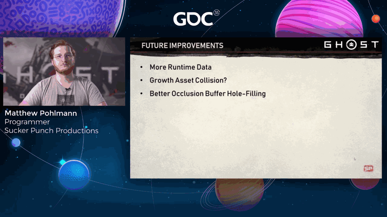
In our experience, fast iteration is required for good results. Users who can’t get feedback and changes immediately are less likely to experiment or spend time polishing. Improving things like expression compilation speed and performing incremental evaluation of expressions over multiple frames would provide for a smoother user experience and even quicker turnaround for live previews.

The current 600-meter hot zone area is okay, but larger would be much better. When authoring an entire forest, you really need to be able to zoom out and get a much larger feel for the space, especially since large ecotopes often border many other ecotopes or terrain features. We’d also like to allow for world-scale editing of the heightmap and remove Maya and that Flux tool I talked about from our workflow entirely.

But we’re going to have to be creative to get that working on a PlayStation hardware. While their existing toolset is great, there are plenty of other things we’d like to offer in the engine that could integrate with these tools. Some prime examples are road and river editing, probably via splines, and cliff authoring. For Ghost, all cliff geometry had to be placed manually.

We’d also like to add or expose additional layers to our terrain expressions and paint applications, like ocean color and ocean foam. Most terrain and growth data is consumed by the tools, and only a minimal subset ends up in the runtime. By making more data available to engine systems, we could create more precise and dynamic systems rather than relying on statically baked content.

Maybe we’ll solve the growth asset collision issue, but honestly, maybe we won’t. The current system seems to work pretty well, and solving this problem would add significant complexity to the growth tool. Our current occlusion buffer algorithms also work pretty well, but we still get disocclusion pops occasionally. I’d really like to shore up the heuristics we’re using to make them more mathematically correct.

Slide 74 — 00:54:29

📌 要点汇总

（过渡内容，无关键要点）

I’d like to thank you all for listening. If you have any questions that I didn’t or couldn’t answer during the talk, feel free to shoot me an email. And we’re also at Sucker Punch. We’re looking for great programmers, so check out our website if you’d like. Thank you.

Slide 75 — 00:54:45

（该幻灯片时间段内未检测到语音内容）